Feb 10, 2014 | Fulldome Curriculum, Gravity, Planets & Moons
A historical lesson in Volume 2 of the Fulldome Curriculum is the astronomical aspect of the Boston Tea Party. As we learn, Colonists, furious at the tea tax, tossed chests of tea into Boston Harbor on the night of December 16, 1773. Eyewitnesses noted that the chests became stuck in the mud adjacent to the ship and piled up in such a way that the Colonists feared the chests wouldn’t float out to sea and might be partially recoverable. The low tide that night (between 6-9 PM local time), which occurred (coincidentally) simultaneously with the raid, was especially low that night.
Although our lesson concentrates on discovering the Moon’s phase that night, a key element is why both high and low tides were so extreme. It turns out that the Moon was close to New Moon phase and perigee that night, making the tides about as extreme as they ever get. So I’d like to concentrate on explaining why tides occur and why the Moon is the major cause of tides and not the Sun.
 The ancients knew that the Moon caused the tides because the tides roughly coincided with the position of the Moon in the sky. The interval between successive high and low tides is ~13 hours, and the high and low tides occurring the next day were approximately one hour later, mimicking the position of the Moon which moved about 13 degrees to the east each day.
The ancients also noted that the greatest tides occurred during New and Full Moons (spring tides) and the least extreme tides occurred at 1st and 3rd quarter (neap tides). But how the Moon caused the tides had to wait until Isaac Newton. I often ask students: “What causes tides on the Earth?” Their answer is always: “The Moon’s gravity pulling on the water of the Earth.” I then ask them, “Then why doesn’t the Sun cause the tides, since its gravitational pull on the Earth is 180 times stronger than the Moon’s (which is why we orbit the Sun and not the Moon!)?”
 The answer is that it’s the Moon’s differential gravitational force on the Earth that causes the tides. The Earth is close enough to the Moon that the Moon pulls considerably harder on the Earth’s near side compared to its far side. The percentage difference between the Moon’s gravitational pull on the Earth’s near side compared to the far side is 6.9%. The Sun, which is so far away from the Earth that it sees the Earth as essentially a point mass, pulls differently on each side of the Earth by a percentage difference of only 0.017%! Ok, most people (students) will buy this, but do NOT understand why the water bulges on both sides of the Earth.
Figure 1 illustrates the strength and direction of the Moon’s gravitational pull on the Earth at New Moon, i.e., the Sun and Moon are in the same direction. This was essentially the phase of the Moon during the Tea Party, i.e., a day or so past New Moon (thin waxing Crescent).
 Determining the differential force experienced by the Earth is equivalent to asking, “What does the Earth actually ‘feel’ due to the Moon’s uneven tugging on it?
We can calculate that by subtracting out the force vector that the Earth experiences at its center from all the other vectors. This is, by definition, the meaning of differential gravitational force.
To illustrate this, Figure 2 shows the inverse center vector’s tail (drawn in orange) placed at the head of each force vector. We will add this inverse vector to all five vectors and illustrate their resultants by white vectors in Figure 3.
For clarity, let’s just look at the resultant differential force vectors in Figure 4.
 As already noted, there is no vector at the center of the Earth because we added its exact inverse so that it canceled out. (That was the point – asking what does the Earth “feel” is a center of Earth force transformation. Sounds cool anyway…) The remaining vectors make sense if you think about each one of them.
The resultant vector on the right occurs because the Moon pulls hardest on the near side, so subtracting the weaker central force resulted in a vector pointing to the right. The resultant vector on the far side to the left will also make sense because the Moon pulls least on that side, so subtracting the larger central force vector resulted in a force pointing to the left! The resultants on the top and bottom occur because of the slightly different directions that the Moon’s force pulls on those points compared to the direct line at the Earth’s center.
If we continued this exercise at 15-degree intervals (instead of 90-degree intervals) around the surface of the Earth, we would have the resultant vectors shown in Figure 5. The locus of all the vector heads has also been drawn in and this egg shape represents the gravitational equipotential of all the tidal forces, i.e., it’s this shape that the water will attempt to emulate.
 Ok, now what? Well, let’s label Boston in the diagram and talk about it – see Figure 6.
Remember that the Moon and Sun are off in the direction towards the right in all the figures. What approximate time is it in Boston in Figure 6? With the Sun highest in the sky, it would be noon. (I hesitate to say “directly over your head,” but you know what I mean.) What tide would the folks in Boston be experiencing at this moment?
The highest bulge is in the direction of the Sun and Moon, so they must be experiencing high tide. Now let’s advance 6 hours to sunset, i.e., let’s turn the Earth counterclockwise by 90 degrees, as depicted in Figure 7. (Pretend that the Moon hasn’t moved in those six hours, so that the tidal bulge is still in the same direction.)
This is essentially the situation during the Boston Tea Party! The Sun had set and the thin crescent Moon was setting. Boston was experiencing low tide at this time (as shown in Figure 7) and it was an especially extreme low tide because the Moon was (coincidentally) close to perigee, so its tidal effects were maximized. So, when would Boston experience its next high tide?
 Approximately 6 hours later, near midnight, when Boston was on the opposite side of the Earth relative to the Sun and Moon. Figure 7 implies that the high tide it experiences on the far side is not as high as the one on the near side, and this is exactly the case with the tides! The one facing the Moon is somewhat higher (by a foot or so) than the one on the far side! Most people don’t know this, since diagrams in books always draw the tidal bulge in equal amounts on both sides of the Earth, but (as you can see in our accurately drawn diagrams) they are wrong!
How do you implement this knowledge in the planetarium? If you understand the above analysis, you can understand that indeed the tides will be in synchronization with the position of the Moon relative to your location. So, if you have New Moon, then high tides at your location are going to occur (approximately) at noon and midnight as in our Boston Tea Party example. This is because New Moon is highest and lowest (near your nadir) in your sky near noon and midnight, respectively.
 Actually the tides lag by about an hour because the water is trying to keep up with the Moon and lags behind its position. Let’s not get too technical! We haven’t even worried about the irregular landforms of the continents and how they complicate the actual tide heights, like at the Bay of Fundy!
What about the tides at Full Moon? Full Moon will behave similarly to New Moon, i.e., high tides will occur when Full Moon is (approximately) highest and lowest in the sky, i.e., midnight and noon.
What about 1st quarter? Again, the principle is exactly the same! When 1st quarter is highest and lowest in the sky, you should be experiencing high tides. 1st quarter is highest at approximately sunset and lowest (near your nadir) at sunrise. Likewise, 3rd quarter is highest and lowest at sunrise and sunset (respectively).
Confused? It’s ok. What you need to do is understand that the tidal bulge (high tide) is always trying to point to the Moon. So high tide will follow the Moon and the Earth “rotates” within the tidal bulging water so to speak. If you carefully work through the explanation and figures above, you should be able to comprehend when to expect high and low tides! If you can convey this to your audiences, they will have re-discovered what the ancients knew and why knowing the position of the Moon in the sky was important to them!
Sep 30, 2013 | Fulldome Curriculum
After years of development, Volume 2 of the Spitz Fulldome Curriculum has been released as a free supplement to all SciDome sites. The curriculum covers a wide gamut of subjects (see contents in sidebar) and gives educators a new library of slides, animations, and scene files to convey both straightforward and complex subjects.
Analemmas

As many of you know, I’m a fan of analemmas because understanding them leads to a wealth of knowledge about orbital dynamics. With Volume 2, we’ve added the ability to draw to scale analemmas on the planet, just like they were drawn on all quality Earth globes in the past.
The analemma is a tracing of the center of the Sun’s specular reflection on a planet as seen from the center of the Sun at the same time each solar day for that planet.
Time and Timekeeping
There are six mini-lessons which can be combined into one super-class on Time and Timekeeping. Breaking these topics into self-contained subprogram cue files allows the user much more flexibility to adapt the curriculum into their own presentations if they so desire.
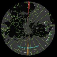
Time Zones

One of our favourite sections is the one on Time Zones which makes use of custom made slides showing time zones on the dome as they would be theoretically drawn, if no humans interfered. Then we crossfade into the real time zones. The Sun can also be moved along the zones to illustrate how time changes relative to universal time – a really cool effect!
New Astronomical Simulations
Steve Sanders, Observatory Administrator at Eastern University, has produced numerous original simulations for Volume 2. These include accurate three-dimensional rotating eclipsing binary stars synchronized with their actual light curves; three-dimensional constellations to clearly show their 3D aspects as seen from other places in the Milky Way; and original depictions of the regression of lunar nodes, and precession of the Earth. One of the most compelling simulations shows exactly why we only have eclipse seasons twice a year separated by approximately six months.
Lincoln Almanac Trial

The regression of lunar nodes animation is used within the Lincoln Almanac Trial lesson to illustrate why the Moon’s high/low seasons were crucial in vindicating Lincoln’s defense of a client in 1857. Lincoln produced an almanac that said that the Moon was setting only three hours after transiting the local meridian – contradicting the witness’s claim that he saw the murder by the light of the moon.
Precession
The Precession video depicts what the precession of the Earth looks like from space and emphasizes that the motion of the equinoxes along the ecliptic is a simple consequence of this gyroscopic motion. The Eclipse video depicts the Earth-Moon system relative to the Sun through the year and wonderfully illustrates how the inclination of the Moon’s orbit causes its New and Full Moon shadows to only lie along the ecliptic during the two eclipse seasons.
You have to see these animations to truly understand how excellent they are! And since they are just mpg files they can also be shown in a classroom setting through a digital video projector.
Planet Locations

One of my primary purposes in planetarium education is to convey to my students straightforward ways to translate what they see in the sky into a fundamental understanding of why they are seeing what they see. This new class exploits the setting Sun’s position to then plot the positions of the other planets onto a curtate orbit chart which each student has on a clipboard.
I have had tremendous success using this method to convey the planets’ positions along the ecliptic to where they actually are in their orbits around the Sun, and the students never look at the skies the same way once they have worked through this class!
I have only touched upon some of the material contained within Volume 2. If you will take the time to peruse the numerous At A Glance scripts you will find an incredibly rich source of new astronomy topics for your audiences.
I’m very excited to have you explore the potential teaching features of Volume 2 with your students! Now it’s time to begin working on Volume 3. If you have any ideas that you’d like to see me create, just email me at dbradstr@eastern.edu.
Sep 30, 2012 | Fulldome Curriculum
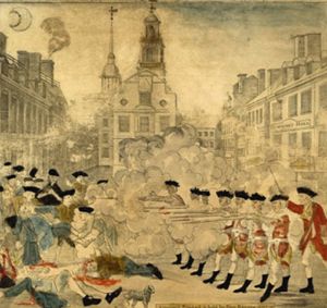
Figure 1: Paul Revere’s depiction of the Boston Massacre
Some of the richest resources of astronomical events and history are the articles of Dr. Donald W. Olson of Texas State University at San Marcos. He has written on an incredible number of topics, including this subject, published in the March 1998 issue of Sky and Telescope, which deals with the Boston Massacre.
The Boston Massacre occurred in 1770. Relations between the colonists and the occupying British troops were very strained, and on the evening of March 5 a group of angry townspeople gathered. They harassed the British guard outside the Town House on King Street, and at 9 PM the British called out more troops to handle the menacing group.
The crowd of colonists threw sticks, snowballs (it had snowed heavily the night before leaving a foot of snow on the ground), and ice at the soldiers. Captain Preston was in front of his men trying to restrain them from losing control, but eventually a shot was fired and then several others rang out haphazardly. When all was said and done, five colonists lie dead or wounded on the ground.

Figure 2: Old State House
The most famous engraving of this incident was made by Paul Revere and is shown in Figure 1.
There are several gross inaccuracies in this engraving as Revere was trying to incite anger and resentment against the British for this incident. (In fact, John Adams would eventually represent the soldiers accused of murder in this confrontation and because of his skill as a lawyer the court found them all innocent!)
Notice that Captain Preston is shown behind his men and they are firing orderly in a volley seemingly at his command. This is a fabrication. Also note that there is no snow on the ground.
The building in the center of the engraving is the Old State House (called the Town House at that time) and it still stands in Boston today along the Freedom Trail as shown in Figure 2. Especially note the strange looking “crescent” Moon in the upper left hand corner of the engraving in Figure 1.
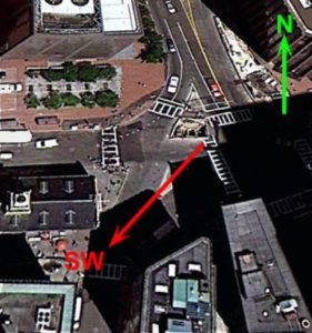
Figure 3: Boston Massacre site with Old State House on left
Here is yet another strange depiction by Revere since the Moon never looks like this in the sky, i.e., a fat “crescent” Moon! Was this yet another fabrication by Revere to emphasize that the Massacre occurred at night, or was his depiction of the phase and placement of the Moon accurate?
To determine this we must first orient ourselves based upon his engraving. We are facing the end of the Old State House in Revere’s engraving. A search on Google Earth shows the orientation of the Old State House (due west from our vantage point in the engraving) and the red arrow shows the location of the Massacre and the direction (southwest) towards the Moon that he drew.
So, what remains for us to determine in the planetarium is what exactly did the Moon look like at 9 PM March 5, 1770 and where was it in the sky? How accurate was Revere in his astronomical depiction? Going to Boston, MA and the proper time and date leads us to the view shown in Figure 4.
Figure 4: 9 p.m. sky over Boston on March 5, 1770 (Moon enlarged for clarity)
We see the Moon is in the approximate position that Revere indicated. What is also interesting is that the approximate surface area depicted in his engraving is correct, although it’s really a waxing gibbous moon and not crescent. (It’s been known for a long time that artists typically drew the Moon as a crescent because it’s more esthetically appealing than a gibbous phase.)
So, although Paul Revere’s propagandist engraving was rife with inaccuracies in order to enrage the colonists, his depiction of the position and brightness of the Moon were fairly close (the crescent phase notwithstanding!).
This fairly bright Moon coupled with a foot of snow on the ground would have given the colonists and soldiers ample light in order to see exactly what they were doing in this most famous initial skirmish which helped lead to the American Revolution.
Feb 28, 2012 | Fulldome Curriculum, Time
Figure 1: Stars added to Sun Distance Spheres
Distance Spheres included in Starry Night allow “Cosmic Zoom” sequences in our domes. However, I also use them to show audiences scale sizes of stars, the Milky Way’s supermassive black hole, and the speed of light.
In a previous article I described the upcoming “Stellar Sizes” minilesson from the Fulldome Curriculum Volume 2. This program compares the sizes of a dozen different stars to each other on the dome. Here’s another captivating way to illustrate stellar scales, but this time compared to the size of the Solar System on the dome making use of Distance Spheres in Starry Night Dome.
I’ve added new Distance Spheres centered on the Sun and made them the appropriate scale according to the sizes of the stars as given in Starry Night and the scientific literature. The stars added as Distance Spheres are shown in Figure 1.
Figure 2: Betelgeuse compared to the Solar System
We can easily add a star’s size to its label name, so as they appear in the dome, their sizes will also show. I’ve colored them appropriately either by temperature or my prejudiced preference. It’s possible to change their opacities so that they look gaseous but you can also see planetary orbits through them, as shown in Figures 2 and 3 which show Betelgeuse and VY Canis Majoris (arguably the largest star known in the Milky Way).
I’ve also added the supermassive black hole that lurks at the center of the Milky Way, which is almost the same size as the star Arcturus. It’s very interesting to see how “small” this 4.3 million solar mass object is compared to the Solar System, as shown in Figure 4.

VY Canis Majoris compared to the Solar System
You can turn various spheres on and off in the dome via SciDome’s “QuickSphere” cue (QS) and or by loading various Starry Night files.
Another useful trick is hidden in a special Distance Sphere which is centered on the Earth, namely the time-varying Radio Sphere. The size of this sphere depends on the date you look at it as it’s expanding at the speed of light. The beginning point in time for this sphere is 12/12/1901 at 14:29:59 UT. So, I’ve set up a Starry Night simulation far enough away from the Earth to see the Moon’s orbit easily with the time stopped.
I tell my audience to watch carefully and they will see the light sphere expand away from the Earth in real time and reach the Moon’s orbit in 1.3 seconds, as seen in Figure 5.
Figure 4: Supermassive Black Hole of the Milky Way compared to the Solar System
You can also increase your elevation to encompass larger volumes of space to watch this sphere expand into the solar system. It’s educational to emphasize that, although light makes it to the Moon in slightly more than one second, it takes minutes to reach the planets, etc.!
I’ve found these to be great tricks for showing students the size of stars and our supermasive black hole compared to the size of our Solar System as well as illustrating the speed of light. I highly recommend that you play with this wonderful new tool in our SciDome teaching arsenal!
Figure 5: Light Sphere after traveling one second, almost to the Moon’s orbit