For the last couple of days, there has been some news coverage of another small asteroid that’s going to fly close to the Earth tonight. This happens fairly often, although it is a little unsettling when it does. We have just passed the 9th anniversary of the discovery of a small asteroid that was on a collision course with Earth in October 2008. That object produced a fresh field of meteorites in Sudan.
NASA illustration of 2012 TC4 near approach
The new asteroid 2012 TC4, was discovered on October 4th, 2012. It flew past Earth on October 12th of that year, 96,000km away. It’s only 13 meters across, and small asteroids like it and the other one tend to be discovered only when they are close enough to the Earth to be visible in large telescopes. Because the orbit of 2012 TC4 is tangent to the orbit of the Earth in October, the only time during the year when Earth and TC4 can be close together is in October. Since that 2012 encounter, the period of TC4’s orbit has been 1.67 years, so we are bound to be close together again after a five-year interval.
After this evening’s encounter, when only 43,000km will separate Earth and TC4, the period of its orbit will be lengthened to 2.06 years. The asteroid orbit will still be tangent to Earth’s orbit in October, and that extra 0.06 of a year will accumulate and may put the asteroid back close to Earth in October 2033 or 2050.
The way Starry Night simulates asteroid orbits in a conventional way depends on those orbits not changing very much. The Keplerian orbital elements model just requires six numbers that describe the orbit of an asteroid around its parent body. Starry Night models these numbers with an accuracy of up to 7 decimal places, and that’s accurate enough to describe asteroids in most of interplanetary space. Keplerian orbits do not simulate the way the Earth’s gravity can deflect the orbit of an asteroid around the Sun, and any asteroid that passes really close to the Earth will be deflected in that way. So the best way for us to simulate TC4’s encounter with Earth in SciDome is unconventional.
Simulating TC4 on SciDome
I have prepared a “Space Missions” file, composed of a set of state vectors from the JPL website that describe TC4’s path for the 8-day period centered on this week’s encounter. It accurately models the way TC4 will sneak as close to Earth as the belt of geosynchronous satellites, and the orbit should be accurate to 0.1km and about 10 seconds in time.
The space missions dataset, and the JPL data format that can make data for it, are originally meant to simulate spacecraft, not asteroids, but the way the data is presented is mostly the same. Although if you “fly to” TC4 in Starry Night, it will look like a space probe and not an asteroid.
If you have a recently updated SciDome, you can get 2012 TC4 on your dome by downloading this zip file, opening it up, then installing “2012 TC4.xyz” on your Preflight computer at the following folder location:
It may be necessary to create a “Space Missions” folder in Sky Data here. If it is, it should be named just so.
If you have an older SciDome, the destination folder for the new file is a little different. Please contact me for directions.
With that done, the next time you run SciDome V7, you ought to be able to find 2012 TC4 by typing it into the search engine field at the top of the pane you choose to use as your “Find” pane. The “Celestial Path” or “Local Path” can be highlighted to show its course across Earth skies, and its “Mission Path” can be highlighted to represent its three-dimensional path through space around the Earth. The position of TC4 will only be simulated during the current 8-day period. If interest in it persists, its new orbit ought to be stable enough to represent with Keplerian elements after everything settles down.
TC4 will be passing through the constellations Aquarius, Capricornus and Sagittarius this evening. I used the JPL data to set up a prediction and make a reservation to use a 150mm online telescope in New Mexico tonight to try and take some images of TC4 as it passes by. We’ll see how it goes. Please feel free to contact me if you would like a little more guidance on installing 2012 TC4 on your SciDome.
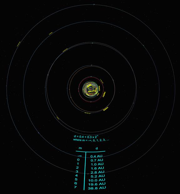
Volume 3 of the Fulldome Curriculum includes a lesson based on the Titius-Bode “Rule.” In this new teaching module we present the orbits predicted by the Titius-Bode relation in a historical timeline compared to the actual planetary orbits to show students why this apparent rule was important in 18th and 19th century astronomy.
The Titius-Bode “Rule” purports to describe an apparent mathematical correspondence in the sizes of the orbits of the classic planets in our Solar System. Although the idea of some kind of relationship had been hypothesized before Johann Daniel Titius and Johann Elert Bode, their publications in 1766 and 1772, respectively, brought this relation into the limelight of astronomical thought, and hence it is named after them.
The idea is that there is a mathematical relationship between each of the orbits of the classic planets. Usually it is presented in the following form:
d=0.4+0.3x2m
… where m = -∞, 0, 1, 2, 3,… and d is the semi major axis of the planet in astronomical units.
Historically, this relationship was believed to be revealing something intrinsic about the positioning of the planets in the Solar System, that there might have been some type of resonance phenomenon within the formation of the planets within the solar nebula. The reason for this belief came out of the astronomical discoveries which were made subsequent to its popularization in the 18th century. To see this in its historical context, let’s set up a table the way it would have been constructed in the late 1700’s:
Interesting results, but the huge gap between Mars and Jupiter posed a real problem!
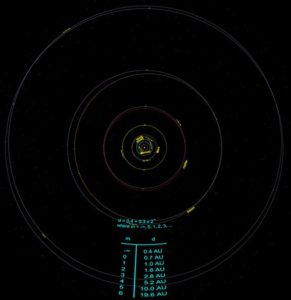
SciDome view showing Uranus’ orbit compared to the Titius-Bode prediction
Shortly after the Titius-Bode “Law” became publicized, William Herschel in 1781 discovered a new planet, Uranus! This was a paradigm changing discovery, but what was just as incredible was that its semi major axis was calculated to be 19.2 AU, nearly doubling the size of the Solar System! Just as remarkable, the next predicted semi major axis from the Titius-Bode “Law” was 19.6 AU, only 2.1% different from the measured size!
This discovery started astronomers thinking that perhaps there was more to the Titius-Bode “Law” than they once thought, that perhaps it wasn’t coincidence but was revealing a yet undiscovered physical relationship within the Solar System. Twenty years later, on the first night of the new century, 1801, Father Giuseppe Piazzi discovered a new “planet,” later named Ceres.
What was truly remarkable about this new planet was that it’s semi major axes was eventually calculated with a new mathematical method by Carl Friedrich Gauss to be 2.8 AU, nearly exactly what the Titius-Bode “Law” had predicted for a planetary body residing in the gap between Mars and Jupiter! Of course soon thereafter many more bodies were discovered to reside within the gap, and by the 1850’s these objects were renamed asteroids.
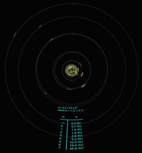
However, the belief in the Titius-Bode “Law” was gaining new proponents, since it seemed to have predicted positions in which Solar System objects were subsequently discovered! The next predicted orbit would lie at 38.8 AU, and the search was on for yet another planet! Sure enough, Neptune was discovered with the aid of Newtonian physics in 1846, but its semi major axis was 30.1 AU, notthe 38.8 AU expected from the Titius-Bode relationship.
SciDome display showing the large discrepancy between Neptune’s orbit (30.1 AU) and the predicted Titius-Bode orbit of 38.8 AU
This large discrepancy led to the virtual abandonment of the Titius-Bode relationship as a physical law. However, it’s interesting to note that when Pluto was discovered in 1930 its semi major axis was determined to be 39.5 AU, very close to the previously expected distance. Of course Pluto has now been relegated to dwarf planet status because of the myriad of new objects which have been discovered in the Kuiper Belt.
The next expected semi major axis from the Titius-Bode relationship is 77.2 AU. And isn’t it interesting that Sedna’s perihelion distance is 76.1 AU, although its semi major axis is a whopping 506.8 AU!
The moral of the story seems to be that although the Titius-Bode relationship has never been convincingly proven to come from physical laws, it is noteworthy historically but also serves to perhaps warn us about jumping to conclusions even though the initial evidence may seem inviting. The Titius-Bode relationship is today such a controversial topic that Icarus, the main professional journal for presenting papers on Solar System dynamics, refuses to publish any articles on the subject!
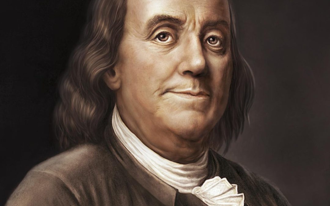
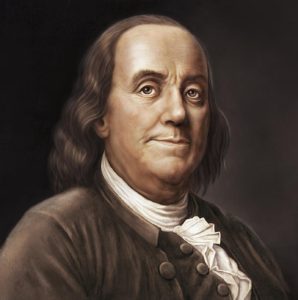
Today is Benjamin Franklin‘s birthday under the calendar we use today, although he was born on the 6th of January of 1706. He was born before the Gregorian calendar reform was implemented in the English-speaking world.
The Gregorian calendar reform adjusted the way that leap years are counted. Instead of observing an intercalary day in February once every four years, the Gregorian observes one such day every four years except when the year is divisible by 100, except when the year is also divisible by 400.
The exact time it takes the Earth to go around the Sun 365.2422 days, not an integer number of days. During the Julian period the remainder was reduced from the 365-day year by adding a leap day every four years. However, the remaining error compounded. The Gregorian calendar uses 97 leap days every 400 years instead of 100 leap days, so the average length of the Gregorian year is 365.2425 days. The Gregorian change also ran a correction to delete the accumulated lag, which had grown to 10 or 11 days.
The new calendar came into force in Roman Catholic states in 1582.
Denmark switched to the Gregorian calendar in mid-February 1700.
The British Empire made the change in 1752.
For any celebrity birthdates you want to celebrate that are older than a certain limit and come from a certain country, it may be important to see if they should be read out as a Julian or a Gregorian date.
If you bring up Starry Night with a date of October 4th, 1582, and advance by one day, you can observe the 10-day correction when the Gregorian calendar was assumed.
The only alternative to observing the ten-day gap that followed in 1582 when looking at earlier dates is to use the proleptic Gregorian calendar, which eliminates the need for a Julian calendar correction when observing past dates. I wouldn’t recommend using the proleptic Gregorian calendar for earlier dates because the people of the time did not use it either, and Starry Night will read out those dates using the Julian.
By 1752, when the British Empire adopted the Gregorian, the accumulated error had grown to 11 days, and the change was reflected in the British colonies that later became the United States. Benjamin Franklin had already been publishing Poor Richard’s Almanac since 1733, and he included a long explanation of the calendar reform in the 1752 edition.
(When Abraham Lincoln used an almanac to show the phase of the moon during the Trial by Moonlight in 1858, as in our Fulldome Curriculum, he was taking a page from one of the most popular kinds of document in the English language other than the Bible.)
The calendar reform of 1752 didn’t catch everyone by surprise, and although the correction was run in September 1752, Franklin had adequate notice before his publication deadline the previous year. The British Parliament passed the new rule as the Calendar (New Style) Act 1750, although the code used for that legislation was “24 Geo. 2 c.XXIII”, meaning it was the 23rd piece of legislation that received royal assent in the 24th year of the reign of King George II. King George had commenced his reign in 1727.
The first point of the new law, before the Julian correction, was to correct the date of the beginning of the legal new year. Although different cultures have strong traditions to begin the new year on January 1st, even now it is impractical for all of our traditions to line up on a single start date: the school year and the NFL season being a couple of examples. The British Empire up to 1752 had observed the start of its legal year on March 25th. The law passed in 1751 corrected the New Year to January 1st at the beginning of 1752, so the official year 1751 was only 282 days long.
Starry Night does not incorporate any of the other weirdness around calendar reform, except that the new year always starts on January 1st, and there is a year Zero in between the BC and CE periods. (ATM-4 does not calculate a Year Zero).
Happy Birthday to Ben Franklin, who was not born on Blue Monday (It was a Sunday in both calendars, and the days of the week have never accumulated an error).
Our ancestors were highly intelligent people who devised ingenious methods to model what they perceived to be reality in the skies. Unfortunately, they came at many of these observations with deep-rooted prejudices and a priori (preconceived) beliefs which shackled their creativity.
Figure 1: Close up of the Ptolemaic system out to the Sun’s sphere
The prevalent, far-reaching belief was that the Earth was immovable and at the center of the universe. Of course we know this is preposterous (even to the point that there is no such thing as a center to the universe), it is still a useful exercise to challenge students to prove, without leaving the Earth or using satellites, that the Earth does indeed rotate and that it revolves about the Sun.
Another a priori assumption was that celestial bodies never stopped moving, as opposed to “earthly” objects which eventually came to a halt. So, when the planets periodically went back and forth in the sky, this was unacceptable and Apollonius of Perga came up with a “solution” that allowed the wanderers to be always moving without stopping by coupling two motions at once. The planets were not simply attached to a mystical sphere (“deferent”) but they were actually attached to a mini-sphere (“epicycle”) which rotated on the larger one.
Figure 2: Mercury’s retrograde path in the Ptolemaic system
In this way planets could move around the sky but intersperse that generally easterly motion with apparent backwards motion (retrograde) when the transparent epicycle carried the planet backwards. The ancients latched on to it and it was greatly preferred to having deferents slow down, stop, go backwards, stop, then resume their original direction.
My colleague David Steelman and I created a program called Epicycles for SciDome that illustrates the main characteristics of the Ptolemaic Geocentric Model. It helps students discover the systemics of the model which can only be explained as “it just has to be that way”. Whenever that is the reasoning, it signals a problem with the theory/model. This will become obvious as we go through this paper.
Let’s first take a close look at the bodies closest to the Earth in the geocentric model, as shown in Figure 1.
The Moon moves the fastest in the sky (and even changes shape!) so it was assumed to be closest to Earth. Placement of Mercury and Venus closer to the Earth than the Sun was problematic. The theory was based upon the idea that those that appeared to move the slowest must be farthest away from Earth. The problem is that the epicycle containing Mercury, the epicycle containing Venus, and the Sun all orbited around the Earth in one year! So their order was reluctantly agreed upon because Mercury moved fastest on it epicycle, Venus next fastest, and of course the Sun had no epicycle (because it never retrograded).
Figure 3: Venus and Mercury’s retrograde paths in the Ptolemaic system
The epicycle sizes are based on arbitrarily assumed distances from Earth. The angles had to match the size of the retrograde loops seen in the sky so, looking at Figure 1, Mercury’s epicycle is tiny compared to Venus’ because Mercury’s retrograde loop is about 52 degrees in extent whereas Venus’ is about 92 degrees! The fact that Venus is farther away than Mercury from the Earth in this model requires it to be considerably larger than one might expect, but these are to scale to create the properly sized retrograde patterns.
As time is progressed a trace can be turned on which shows the retrograding patterns of the planets. Figure 2 shows a close up of Mercury and Figure 3 that of Venus.
When I ask students if they see anything peculiar as time progresses, eventually someone notices that the centers of the epicycles of Mercury and Venus are exactly and always lined up with the line connecting the Earth and Sun (the Earth-Sun Line). What explanation would the ancients have given for this? “It just has to be this way for this model to work.” Red flag number 1 that there’s something wrong with this theory.
Figure 4: The planets beyond the Sun’s sphere
Of course we know that in the Copernican heliocentric model we don’t need epicycles to cause Mercury and Venus to wobble back and forth around the Sun because they are simply closer to the Sun than Earth and they orbit the Sun. In fact, Copernicus was the first to completely untangle the motions of Mercury and Venus from the Sun’s motion.
This confusion is one rarely-discussed reason why the Copernican heliocentric model was so appealing. It unambiguously separated the motions of Mercury and Venus and even established, for the first time, their orbital periods around the Sun (88 days and 225 days, respectively).
Now observe the planets beyond the Sun, as shown in Figure 4. As we advance time another strange systematic displays itself, although this one is a lot more challenging to pick out. The Earth-Sun Line is always parallel to the planet’s epicycle radius! You can easily see this in Figure 4 now that you know to look for it.
Again, the ancients noted this “coincidence” but could never explain it other than “it has to be this way for the model to work.” Another red flag has raised itself in the flawed Ptolemaic model! The basic reason for this “coincidence” is because the retrograde motion of each planet is a function of its position relative to the Earth in its own orbit. Since we’re locking down the Earth and moving the Sun, it’s the orientation of the Earth-Sun Line that is the determining factor as to when planets exhibit their retrograde motions.
Figure 5 – The retrograde paths of the planets beyond the Sun’s sphere
When the planets leave breadcrumbs (see Figure 5) their retrograding paths become obvious. Again, the model has been carefully defined to accurately recreate the width of the retrograde loops as well as their frequency.
This is a fun and thought provoking lesson for my students because it demonstrates how intelligent and clever the ancients were in mimicking celestial motions, but it also shows how preconceived notions can weigh one down and severely complicate the model. It also clearly points out that when certain “features” of a model have no other explanation than “it has to be that way for the model to work” that the model is most likely flawed or incorrect at its core. But having the Earth move was a huge paradigm shift, and it took over 1500 years to overthrow it!
Figure 1: Page from the original printing of Sidereus Nunicius showing Galileo’s sketches of the Medicean Moons
In many of our astronomy classes, we discuss the importance of Galileo’s first telescopic observations in eventually overthrowing the Ptolemaic geocentric system. His first observations were relayed to the public in his short book Sidereus Nuncius, which is Latin for The Starry Messenger (or arguably, The Starry Message). In it he relates his observations of the Moon, the myriad of new stars he observed (with sketches of the Pleiades and Praesepe regions), and the Moons of Jupiter.
He originally called these the Medicean Stars, a call out to his potential benefactors, the four Medici brothers (the book itself was dedicated to one of them who had been a former pupil). Seeking for funds for your science… things really haven’t changed very much in 400 years…
With Starry Night, SciDome can easily reproduce the date and situations of Galileo’s observations. Others have done this in the past, and I refer you to the excellent article by Enrico Bernieri called “Learning from Galileo’s Errors” published in the Journal of the British Astronomical Association, 122, 3 (2012) which goes through his observations in detail and discusses the errors which Galileo made.
I also highly recommend the Wikipedia article on Sidereus Nuncius as an excellent starting point in building your background information on Galileo’s first telescopic observations. In addition, Ernie Wright has graphically reproduced Galileo’s observations and placed them online in an excellent web presentation.
With the incredible talent of Steve Sanders (Eastern University Observatory Administrator), I have created a minilesson for Volume 3 of the Fulldome Curriculum which reproduces all of Galileo’s published observations of the Medicean moons.
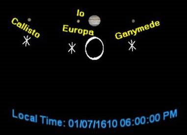
Figure 2: SciDome presentation of Galileo’s first Jupiter observations from January 7, 1610 from Padua, Italy.
Using Padua, Italy as our observation location and the approximate times given for each observation in Sidereus Nuncius, we begin with the close-up view of Jupiter on the dome as seen on January 7, 1610 at approximately 6 PM local time. Next we place a slide of the view as drawn by Galileo in Sidereus Nuncius below the view to show just how accurate Galileo was in his sketches. The labels of the Galilean moons are then displayed.
Note that although all four moons presented themselves, Io and Europa were too close together to be resolved by Galileo’s homemade 20X telescope which suffered also from chromatic and spherical aberration. This is an important fact to remember, because essentially all of the “errors” which we will find in comparing his sketches to the actual viewing circumstances were because of his lack of resolution.
We proceed by advancing time in Starry Night so that the audience can watch the dance of the moons around Jupiter and stop at the next observations of Jupiter as recorded by Galileo, on January 8, 1610. Then his sketch of this configuration is displayed, and again we note the accuracy of his rough sketches.
The minilesson continues in this fashion, showing the moons moving from date to date and then presenting 21 successive sketches by Galileo as presented in Sidereus Nuncius. Galileo concluded after four nights of observations that these tiny “stars” were indeed most likely satellites of Jupiter, which was of momentous importance because it was the first time that moons had been discovered around another body.
It also indicated that a planet could move and moons “stay up with it” despite its motion, an Aristotelian argument once offered to discount that the Earth could be moving because, if it did, how could the Moon know enough to keep up with it? Obviously Jupiter had at least four moons and they had no problem staying with it!
I have found that going through many of these configurations with my students greatly enhances their appreciation of Galileo and the great discoveries that he made despite the limitations of his equipment. Presenting this minilesson engages students in the realization that Galileo was both an excellent and honest observer as well as a genius. His observations helped to lead to the downfall of the geocentric universe and the eventual acceptance of the heliocentric model