Nicolaus Copernicus’ (1473 – 1543) paradigm-changing work de Revolutionibus Orbium Coelestium (On the Revolutions of the Celestial Spheres) famously laid the groundwork for the overthrow of the geocentric universe that had held sway for millennia. But what many people are not aware of is that Copernicus’ heliocentric system allowed for the first scale model of the entire known solar system in terms of the size of the Earth’s orbital radius.
What I find most incredible is that the values he determined, despite assuming incorrectly that the planets’ orbits must be circular with the planets traveling at constant orbital speed, are very close to the modern-day measurements (shown in Table 1).
In my never-ending quest to create meaningful and engaging planetarium curriculum, Clint Weisbrod and I have developed the ability to reproduce Copernicus’ method using SciDome and new features in Starry Night which allow us to do solar system geometry.
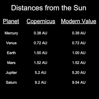
Table 1 – Results of Copernicus’ model versus modern values.
We begin by looking at the planets closer to the Sun than the Earth, the inferior planets Mercury and Venus (first denoted as such by Copernicus). Figure 1 shows the configuration for greatest elongation of Venus. By definition, this will occur when Venus appears to be the farthest away from the Sun as seen from Earth.
Via Euclid’s geometry we can prove that when Venus is at greatest elongation the angle at the position of Venus has to be exactly 90°. The line of sight from Earth to Venus must be tangent to Venus’ orbit, otherwise the line of sight would intersect the orbit in two places, both of which would display smaller angular separations from the Sun. The elongation angle θ is measured from the Earth as the angle between Venus and the Sun.
Knowing θ and that the angle at Venus is 90°, we can solve all sides of the triangle if we know one side of the triangle. Alas, we do not know any of the lengths, but if we define the distance from the Earth to the Sun (the hypotenuse) as 1 astronomical unit (1 AU), then we can immediately calculate the side of the triangle opposite the elongation angle θ as
Venus distance from Sun = (1 AU) sin θ
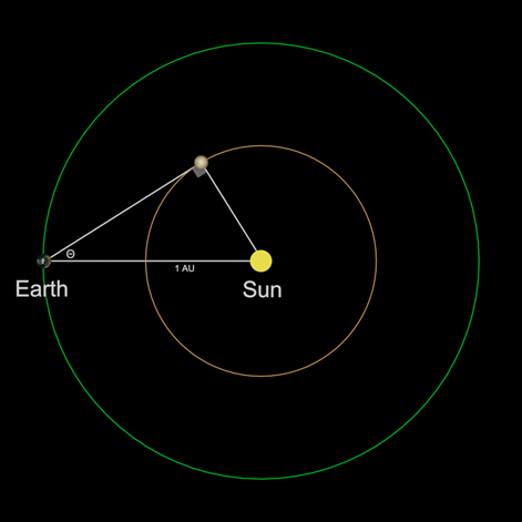
Figure 1 – The geometry (greatest elongation) of inferior planet distances from the Sun.
Figure 2 shows this configuration as seen from a top-down view of the Solar System in Starry Night using the new Copernican Method lines.
The value of the radius of the orbit of Venus (again assuming a circular orbit) is
Venus distance from Sun = (1 AU)sin(45.9°) = 0.72 AU
This is a remarkably accurate result, mostly due to Venus’ nearly circular orbit! The results for Mercury are not as accurate, but of course Mercury’s orbit is far from a circle. However, if enough measurements are made of multiple greatest elongations, the average will come out to be a fairly close estimate to the modern-day value.

Figure 2 – The Copernican Method lines for Venus in SciDome.
What’s awesome about the new feature in SciDome is that we can actually display the Copernican Method lines as seen from Earth as well as from space, as shown in Figure 3.
The line drawn between Venus and the Sun (just below the horizon) also displays the angular separation of the two bodies (45.9°) and the angle at Venus is the angle made between that line and the Earth’s line of sight (89.9° – close enough to 90° for government work).
The greatest elongation angle (45.9°) can be measured (in modern times) using a sextant (invented in 1715), so this new Copernican Method lines feature allows us to draw “sextant measurement lines” between the Sun and the planets.
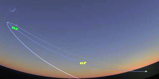
Figure 3 – Venus’ greatest eastern elongation as seen from Philadelphia on August, 15, 2018.
Determining the sizes of the orbits of the planets further from the Sun than the Earth—the superior planets—is not quite so straightforward. The method is explained below, remembering again that we’re assuming the orbits are all circular and the planets are moving at constant orbital speeds.
Figure 4 shows the geometry of the situation for superior planets. We begin by noting the date (Julian Date) of an opposition of the planet, when the planet and the Sun are on opposite sides of the Earth—the superior planet would rise when the Sun sets, and be highest in the sky (on your local meridian) at midnight. We then wait and observe the planet until it is 90° from the Sun, a position Copernicus defined as quadrature.
We calculate the number of days that have passed since opposition, and this will allow us to calculate how many degrees each planet has traversed in their respective orbits. For example, the Earth takes 365.2422 days to cover 360° (again, we’re assuming circular orbits and constant orbital velocity) so it will move
![]()
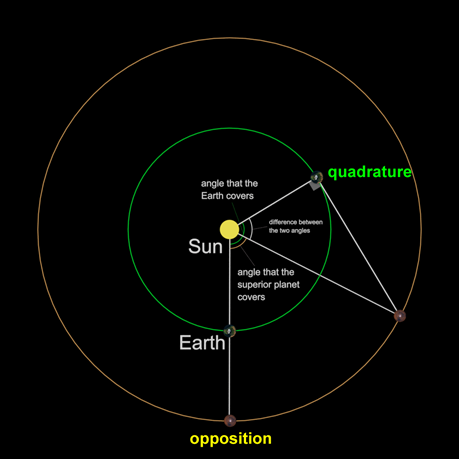
Figure 4 – The geometry of measuring the size of the orbits of the superior planets.
A similar calculation can be done for all the planets since Copernicus had calculated the sidereal periods of all the visible planets (see the Synodic Periods minilessons in Volume 3 of the Fulldome Curriculum). For example, Jupiter’s sidereal period is 4332.59 days yielding an angular rate of travel in its orbit of 0.0831 deg/day.
Since we know how many days it took for the planets to reach quadrature from opposition, we can immediately calculate how many degrees each planet traveled in their respective orbits. The Earth will travel a greater angle in its orbit in this time, and the difference between these two angles is the angle θ shown in Figure 5.
Assuming that the distance from Earth to the Sun is 1 AU, we can calculate the distance from the Sun to Jupiter (the hypotenuse of the triangle in Figure 5) as
![]()
So, what Earth observers would need to do is to measure the number of days from the opposition of a planet to the next quadrature, calculate the difference in degrees traveled between the two planets, and then take the reciprocal of the cosine of that angle to calculate the superior planet’s distance from the Sun.
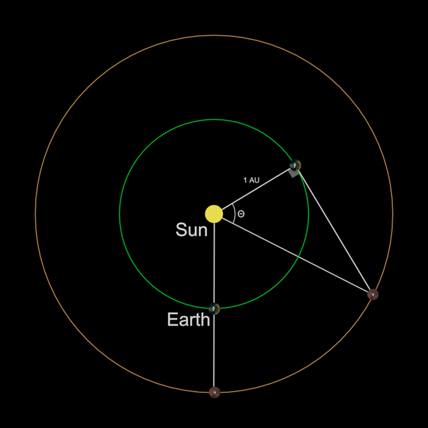
Figure 5 – The quadrature triangle to solve for Jupiter’s distance from the Sun.
In the case of Jupiter, one set of measurements placed opposition on May 9, 2018 (JD 2458247.75) and the following quadrature on August 6, 2018 (JD 2458337.492), for a difference in days of 89.74. This value, multiplied by the difference in angular velocities between Earth and Jupiter, yielded a θ = 81.0°. This resulted in an orbital radius for Jupiter of 6.41 AU, whereas the modern value is 5.20 AU (a 23% difference). The view from Earth of this quadrature is shown in Figure 6.
At first glance, this value seems to be significantly off from the modern value…and it is! Have we made a mistake, or is this yet another opportunity to encourage our students to think? What assumptions have we made that are probably not accurate? We (as did Copernicus) assumed circular orbits and constant orbital velocities, and neither of these assumptions is correct for any of the planets!
So how can we use this method and the (wrong) assumption of circular orbits and constant orbital velocities to arrive at relatively accurate values for the sizes of the superior planets’ orbits?
The answer is to take multiple measurements over at least one orbital cycle of the planet in order for the answers to average out to some median value which indeed will approach the modern-day value. I did this for Jupiter taking 11 successive opposition-quadrature pairs over one 11-year cycle of its orbit from 2007 to 2018. When I averaged these 11 determinations I obtained a value of 5.46 AU, an error of only 5% from the modern value.
Don’t see this as a problem but rather as a very teachable moment for your students. You might challenge them as a class to take multiple measurements of successive opposition and quadrature pairs and they can watch for themselves how the values average out to close to the modern-day value. They can see for themselves how the errors introduced by our assumptions of circular orbit and constant orbital velocities can be minimized (but not eliminated) by multiple observations.
It’s appropriately mind-blowing to see the genius of Copernicus through these observations that your students can now undertake for themselves in the SciDome planetarium! They will gain a much greater understanding of how Copernicus created his solar system scale model, as well as see how these measurements could actually be made from the ground.
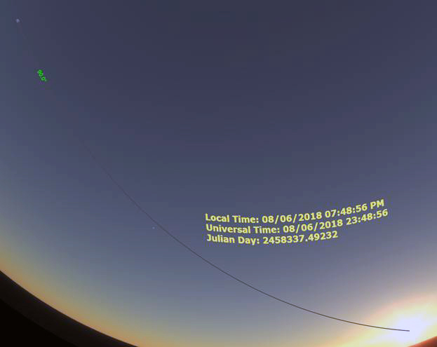
Figure 6 – The quadrature of Jupiter as seen from Philadelphia on August 6, 2018.