Nicolaus Copernicus’ (1473 – 1543) paradigm-changing work de Revolutionibus Orbium Coelestium (On the Revolutions of the Celestial Spheres) famously laid the groundwork for the overthrow of the geocentric universe that had held sway for millennia. But what many people are not aware of is that Copernicus’ heliocentric system allowed for the first scale model of the entire known solar system in terms of the size of the Earth’s orbital radius.
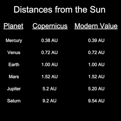
What I find most incredible is that the values he determined, despite assuming incorrectly that the planets’ orbits must be circular with the planets traveling at constant orbital speed, are very close to the modern-day measurements (shown in Table 1).
In my never-ending quest to create meaningful and engaging planetarium curriculum, Clint Weisbrod and I have developed the ability to reproduce Copernicus’ method using SciDome and new features in Starry Night which allow us to do solar system geometry.
Table 1 – Results of Copernicus’ model versus modern values.
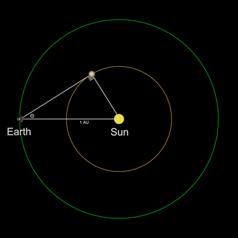
We begin by looking at the planets closer to the Sun than the Earth, the inferior planets Mercury and Venus (first denoted as such by Copernicus). Figure 1 shows the configuration for greatest elongation of Venus. By definition, this will occur when Venus appears to be the farthest away from the Sun as seen from Earth.
Via Euclid’s geometry we can prove that when Venus is at greatest elongation the angle at the position of Venus has to be exactly 90°. The line of sight from Earth to Venus must be tangent to Venus’ orbit, otherwise the line of sight would intersect the orbit in two places, both of which would display smaller angular separations from the Sun. The elongation angle θ is measured from the Earth as the angle between Venus and the Sun.
Knowing θ and that the angle at Venus is 90°, we can solve all sides of the triangle if we know one side of the triangle. Alas, we do not know any of the lengths, but if we define the distance from the Earth to the Sun (the hypotenuse) as 1 astronomical unit (1 AU), then we can immediately calculate the side of the triangle opposite the elongation angle θ as
Venus distance from Sun = (1 AU) sin θ
Figure 1 – The geometry (greatest elongation) of inferior planet distances from the Sun.
Figure 2 shows this configuration as seen from a top-down view of the Solar System in Starry Night using the new Copernican Method lines.
The value of the radius of the orbit of Venus (again assuming a circular orbit) is
Venus distance from Sun = (1 AU)sin(45.9°) = 0.72 AU
This is a remarkably accurate result, mostly due to Venus’ nearly circular orbit! The results for Mercury are not as accurate, but of course Mercury’s orbit is far from a circle. However, if enough measurements are made of multiple greatest elongations, the average will come out to be a fairly close estimate to the modern-day value.
Figure 2 – The Copernican Method lines for Venus in SciDome.
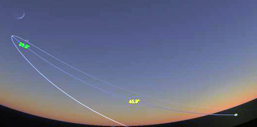
What’s awesome about the new feature in SciDome is that we can actually display the Copernican Method lines as seen from Earth as well as from space, as shown in Figure 3.
The line drawn between Venus and the Sun (just below the horizon) also displays the angular separation of the two bodies (45.9°) and the angle at Venus is the angle made between that line and the Earth’s line of sight (89.9° – close enough to 90° for government work).
The greatest elongation angle (45.9°) can be measured (in modern times) using a sextant (invented in 1715), so this new Copernican Method lines feature allows us to draw “sextant measurement lines” between the Sun and the planets.
Figure 3 – Venus’ greatest eastern elongation as seen from Philadelphia on August, 15, 2018.
Determining the sizes of the orbits of the planets further from the Sun than the Earth—the superior planets—is not quite so straightforward. The method is explained below, remembering again that we’re assuming the orbits are all circular and the planets are moving at constant orbital speeds.
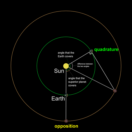
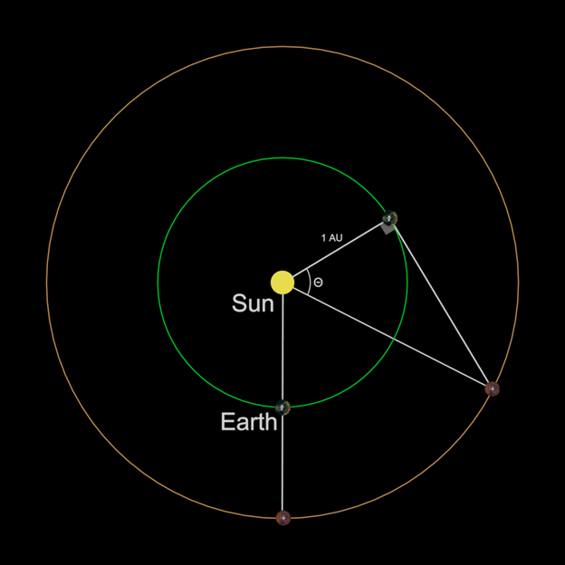
Figure 4 shows the geometry of the situation for superior planets. We begin by noting the date (Julian Date) of an opposition of the planet, when the planet and the Sun are on opposite sides of the Earth—the superior planet would rise when the Sun sets, and be highest in the sky (on your local meridian) at midnight. We then wait and observe the planet until it is 90° from the Sun, a position Copernicus defined as quadrature.
We calculate the number of days that have passed since opposition, and this will allow us to calculate how many degrees each planet has traversed in their respective orbits. For example, the Earth takes 365.2422 days to cover 360° (again, we’re assuming circular orbits and constant orbital velocity) so it will move
Figure 4 – The geometry of measuring the size of the orbits of the superior planets.
A similar calculation can be done for all the planets since Copernicus had calculated the sidereal periods of all the visible planets (see the Synodic Periods minilessons in Volume 3 of the Fulldome Curriculum). For example, Jupiter’s sidereal period is 4332.59 days yielding an angular rate of travel in its orbit of 0.0831 deg/day.
Since we know how many days it took for the planets to reach quadrature from opposition, we can immediately calculate how many degrees each planet traveled in their respective orbits. The Earth will travel a greater angle in its orbit in this time, and the difference between these two angles is the angle θ shown in Figure 5.
Assuming that the distance from Earth to the Sun is 1 AU, we can calculate the distance from the Sun to Jupiter (the hypotenuse of the triangle in Figure 5) as
So, what Earth observers would need to do is to measure the number of days from the opposition of a planet to the next quadrature, calculate the difference in degrees traveled between the two planets, and then take the reciprocal of the cosine of that angle to calculate the superior planet’s distance from the Sun.
Figure 5 – The quadrature triangle to solve for Jupiter’s distance from the Sun.
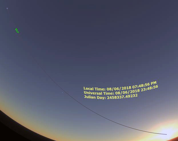
In the case of Jupiter, one set of measurements placed opposition on May 9, 2018 (JD 2458247.75) and the following quadrature on August 6, 2018 (JD 2458337.492), for a difference in days of 89.74. This value, multiplied by the difference in angular velocities between Earth and Jupiter, yielded a θ = 81.0°. This resulted in an orbital radius for Jupiter of 6.41 AU, whereas the modern value is 5.20 AU (a 23% difference). The view from Earth of this quadrature is shown in Figure 6.
At first glance, this value seems to be significantly off from the modern value…and it is! Have we made a mistake, or is this yet another opportunity to encourage our students to think? What assumptions have we made that are probably not accurate? We (as did Copernicus) assumed circular orbits and constant orbital velocities, and neither of these assumptions is correct for any of the planets!
So how can we use this method and the (wrong) assumption of circular orbits and constant orbital velocities to arrive at relatively accurate values for the sizes of the superior planets’ orbits?
The answer is to take multiple measurements over at least one orbital cycle of the planet in order for the answers to average out to some median value which indeed will approach the modern-day value. I did this for Jupiter taking 11 successive opposition-quadrature pairs over one 11-year cycle of its orbit from 2007 to 2018. When I averaged these 11 determinations I obtained a value of 5.46 AU, an error of only 5% from the modern value.
Don’t see this as a problem but rather as a very teachable moment for your students. You might challenge them as a class to take multiple measurements of successive opposition and quadrature pairs and they can watch for themselves how the values average out to close to the modern-day value. They can see for themselves how the errors introduced by our assumptions of circular orbit and constant orbital velocities can be minimized (but not eliminated) by multiple observations.
It’s appropriately mind-blowing to see the genius of Copernicus through these observations that your students can now undertake for themselves in the SciDome planetarium! They will gain a much greater understanding of how Copernicus created his solar system scale model, as well as see how these measurements could actually be made from the ground.
Figure 6 – The quadrature of Jupiter as seen from Philadelphia on August 6, 2018.
Three long-awaited fulldome astrophysics apps created by Dr. David H. Bradstreet are now available for purchase and immediate download for installation on SciDome systems. Tides, Newton’s Mountain and Epicycles are selling for $200 individually or $500 for all three.
REQUIRES WINDOWS 7 ON THE RENDERBOX COMPUTER. Multi-projector systems must be based on Scaleable – not compatible with EasyBlend.
These programs teach the difficult concepts of tides, orbital motion, and epicycles in unique ways on your dome. All three programs are completely controllable via an intuitive interface on your Preflight computer. In addition, Tides is controllable via SciTouch for a seamless teaching experience for your audience.
The respective At A Glance teaching guides are all available for free download if you’d like to preview what you can do with these unique Fulldome interactive programs:
48 years ago last week Apollo 11 landed on the Moon. There is another anniversary last week that seems appropriate to mention at this point: On July 20th of 1925 the greatest scene in American legal history took place, and it was an astronomy lesson.
You’re probably familiar with the play Inherit the Wind, which was based on the Scopes Monkey Trial. In the summer of 1925, more specifically on July 20th, on the courthouse lawn in Dayton, TN, Clarence Darrow had William Jennings Bryan on the witness stand to respectively challenge and defend the state’s Butler Act that prohibited public school teachers from denying the Biblical account of the origin of humanity.
Darrow and Bryan were agreed on the terms of the Earth being a sphere, and that the Earth orbits around the Sun and not the other way round. Therefore it was necessary for them to interpret the biblical passages that seemed to indicate that the Earth was flat and that the Sun stopped at midday for Joshua.
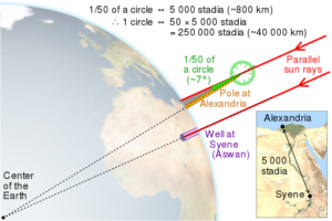
Illustration of Erastothenes’ method by CMG Lee. CC BY-SA 4.0
That the Earth was round, and that the Earth was turning and the Sun was at the axis of the solar system was not difficult to accept in 1925. People were familiar with Eratosthenes’ 3rd-Century-BC experiment in Egypt to estimate the circumference of the Earth (252,000 stadia.) They were also familiar with the great American novelist Washington Irving’s biography of Christopher Columbus, which laid out Columbus’ theory of the roundness of the Earth and his discovery of America obstructing the route to India.
That the Earth was round was also not difficult to accept in the 1480s when Columbus solicited the crowned heads of Europe to fund his voyage to India. It’s just a simplification of Washington Irving’s biography of Columbus to say that Columbus was trying to prove that the Earth was round and that his opposites held that it was flat. In the 4th chapter of the biography, the author puts Columbus in front of the School of Salamanca where he is criticized for the way he contradicts classical dogma from Saint Augustine in the 4th Century AD concerning the “Doctrine of Antipodes“.
In modernity, the antipodes are the geographic point opposite one’s position on the globe, but these medieval Antipodes were the mythical people supposed to inhabit the southern hemisphere who walked upside down (antipode meaning “reversed feet.”) but Saint Augustine did not dispute that the Earth was round:
“As to the fable that there are Antipodes, that is to say, men on the opposite side of the earth, where the sun rises when it sets to us, that is on no ground credible. And, indeed, it is not affirmed that this has been learned by historical knowledge, but by scientific conjecture, on the ground that the earth is suspended within the concavity of the sky, and that it has as much room on the one side of it as on the other: hence they say that the part which is beneath must also be inhabited. But they do not remark that, although it be supposed or scientifically demonstrated that the world is of a round and spherical form, yet it does not follow that the other side of the earth is bare of water; nor even, though it be bare, does it immediately follow that it is peopled.”
Columbus’ critics in the Inquisition, if any, subscribed to dogma that the Earth was round but that human civilization was limited to the temperate zone of the northern hemisphere by the Torrid Zone at the equator. That there was a corresponding southern temperate zone in the southern hemisphere, but that humans created in Genesis could not exist there because the Garden of Eden was in the north and the Torrid Zone was impassable or nearly so. That navigation to get there wasn’t easy because there was no North Star in the south, and the Doldrum Belt made headway under sail to the opposite end of the Earth impossible. The 1st-Century-BC Roman writer Cicero had written about the impassable Torrid Zone in an item called the Dream of Scipio, which is a good basis for an old-timey planetarium show in itself.
“Moreover you see that this earth is girdled and surrounded by certain belts, as it were; of which two, the most remote from each other, and which rest upon the poles of the heaven at either end, have become rigid with frost; while that one in the middle, which is also the largest, is scorched by the burning heat of the sun. Two are habitable; of these, that one in the South—men standing in which have their feet planted right opposite to yours—has no connection with your race: moreover this other, in the Northern hemisphere which you inhabit, see in how small a measure it concerns you! For all the earth, which you inhabit, being narrow in the direction of the poles, broader East and West, is a kind of little island surrounded by the waters of that sea, which you on earth call the Atlantic, the Great Sea, the Ocean; and yet though it has such a grand name, see how small it really is!”
It is true that Columbus was trying to sail around the world to reach India, and that he had underestimated the circumference of the Earth due to a conversion error from Eratosthenes: by the 15th Century, the value of 252,000 stadia was remembered, but the value of a stadion was uncertain, and Columbus used the wrong value. Therefore the Earth seemed smaller, and globes of the Earth from that period show the East Indies on the western edge of the Atlantic Ocean.
Columbus was convinced that the Torrid Zone was not a barrier to travel. Earlier in his career he had sailed to West Africa, almost to the Equator. The first European transit of the Cape of Good Hope (which is in the southern temperate zone) into the Indian Ocean was by the Portuguese navigator Bartolomeu Dias in 1488, two years after Columbus’s first unsuccessful examination at Salamanca.
This 1492 globe of the Earth is under a Creative Commons licence, so feel free to demonstrate it via its own API. It could be converted and wrapped around the Earth in Starry Night, but I don’t feel ready make the final product available for SciDome at this time due to the rights.
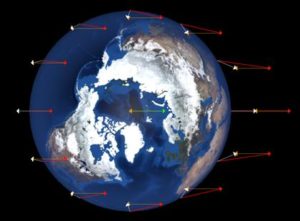
However, there are lots of ways to use SciDome to demonstrate that the Earth is round. The upcoming total solar eclipse is one event that is not easy for flat-earth believers to explain, when its occurrence is so accurately predicted with established science. Performing Eratosthenes’ experiment in SciDome is not difficult, by displaying the sky above his two observing stations in Alexandria and Aswan at local noon on June 21st with the Local Meridian switched on with graduations.
Now that we have established that the roundness of the Earth was accepted by both sides in the 1925 Scopes Trial, and that the roundness of the Earth was accepted by both Columbus and his critics (admitting serious gaps in the knowledge of both sides) and by the ancient Greeks, I hope that we can help elevate current concerns about the Earth being flat. I understand that a large billboard was recently used in suburban Philadelphia next to the freeway to state “Research Flat Earth”. And when we argue against modern flat-earth believers, we should not compare their belief to Columbus’s critics, and commit another simplification of the actual story.
Novae and supernovae are among the most energetic phenomena encountered in the galaxy. Planetarium educators can simulate a number of historical nova and supernova events on SciDome using Starry Night Dome Version 7.
The following 10 transient objects can be investigated in Starry Night 7’s “Historical Supernovae” database on’s :
SN 1987A (Progenitor: Sanduleak -69° 202)
Supernova 1680 (Cassiopeia A)
SN 1604 (Kepler’s Star)
SN 1572 (Tycho’s Star)
SN 1181
SN 1054 (Crab Nebula)
SN 1006
SN 393 (G347.3-0.5)
SN 386 (G11.2-0.3)
SN 185 (RCW 86)
Each of these supernova simulations behave in one of two ways on the dome.
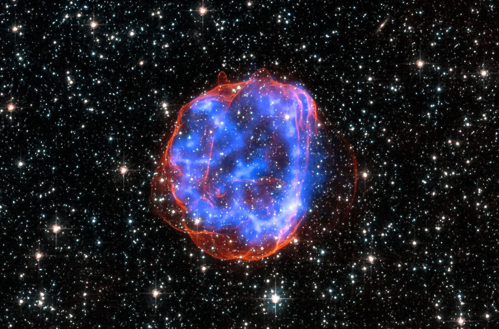
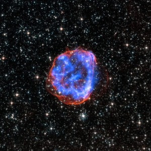
The supernovae of the years 1987, 1604, 1572, 1181, 1054 and 1006 in the Common Era were all relatively well-studied when they were visible, and their positions have been correlated with current supernova remnants. These objects are best treated in SciDome: if you look at the sky on the date they appeared and in the correct position, toggling backward and forward several days, the “Guest Star” phenomenon makes the supernova pop into existence, flare up slightly, and then fade away over the course of several months.
The supernovae of the years 1680, 393, 386 and 185 were not well-observed at the time we estimate they exploded due to interstellar dust blocking their light, the difficulty of keeping reliable extremely old observing records, etc. However, some unconfirmed observing reports claim they were observed, and their positions correlate well with supernova remnants or pulsars detected with X-ray telescopes. With no firm dates or estimated brightnesses, it’s appropriate that their positions should be marked, but these four objects do not flare up and then dim out like the first six. There are also photos of the supernova remnants docked in position over these transients in Starry Night.
How about adding objects to this database manually? That’s not so hard, and there are several candidates that have similarities to historical supernovae (although the above ten are the only recorded historical supernovae that have been as bright as the brightest stars).
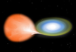
Artist’s conception of a white dwarf accreting hydrogen from a larger companion
If a supernova is a star that explodes completely, a nova is a star that is only partly exploding. There are a few different theories to describe the processes in a nova star. The most common is that a white dwarf star and a normal star are orbiting each other, and the normal star is close enough to deposit some outflowing gas on to the surface of the white dwarf. The gas builds up on the surface of the white dwarf star until it becomes unstable and explodes. The white dwarf star survives the explosion. These novae can even re-occur once the gas builds up again.
Today is the 99th anniversary of the appearance of the “Victory Star”, also known as Nova Aquilae 1918 or V603 Aquilae. For several days this star was the brightest nova in the age of the telescope, magnitude -0.5, as bright as the brightest stars. It faded back to obscurity quickly. It was known as the Victory Star because some saw it as a portent of the end of the Great War. Also, in an extreme coincidence, it appeared on the same day in June 1918 as a total eclipse of the Sun was seen from coast to coast across the United States.
The file that encodes the Historical Supernovae database is in the Sky Data folder for Starry Night 7 on both Preflight and Renderbox. This feature is not available in Starry Night 6. To make a change, both files need to be edited in an identical fashion.
Here is the code that can simulate the Nova 1918 star by pasting into a new “11th” paragraph:
The Right Ascension and Declination (RA and Dec) co-ordinates of the new star have to be entered in decimal hours and decimal degrees. The values in the line with the tag “00011_RA_Dec_DistanceLY” are accurate to put the nova in western Aquila several degrees above the asterism of stars that makes up the “foot” of the Eagle.
Some of the above values are just copied from an earlier part of the file, but the observing period, expressed in Julian dates, is shorter than for a supernova. There are only 248 days between the date 2421752 (representing June 8, 1918) and 2422000 when we can estimate the new star had dimmed below the threshold of visibility.
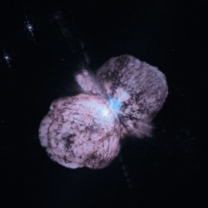
The Homunculus Nebula, surrounding Eta Carinae
There are several other nova stars that can be shoe-horned into this database. For example, the extremely massive star Eta Carinae is currently quite dim and surrounded by an emission nebula, but it is studied so well now because for many years in the mid-19th century its brightness fluctuated wildly up and down, and for some time it was the 2nd-brightest star in the sky.
If future predictions are just an extension of history, perhaps we can use SciDome to get ahead of a possible nova that could flare up in about five years from now. KIC 9832227 is a contact binary star in Cygnus, like the one on the cover of Dr. Bradstreet’s Spitz Fulldome Curriculum Volume 2, and a prediction was made in January of this year that at some time in about 2021 or 2022 the two stars will coalesce together and outburst in brightness. Because the two stars are whirling around each other every 11 hours, due to uncertain mixing and modeling, the error bars make it difficult to accurately predict this “future historic nova”, but it could happen, and we can even try and get the drop on it.
Witnessing a total solar eclipse could change your life. Unpredicted eclipses have changed the progression of historical events. The unexpected environmental effects of a sudden darkness at midday can be very unsettling to people and animals alike.
On July 29, 1878, Thomas Edison observed the total eclipse of the Sun as part of Henry Draper’s Expedition to Rawlins, Wyoming Territory. (Although this year’s total eclipse will pass through Wyoming, the City of Rawlins will be some distance south of the total path this time.) Edison was there to test a new invention that could detect infrared light and estimate the temperature of objects remotely, and he planned to try and estimate the heat of the Sun’s corona while the solar photosphere was blocked by the Moon.
Edison’s preparations for the eclipse were not as cautious as they should have been. Because total eclipses happen close to home so very rarely (2017 is the first year that the totality has appeared in US skies since 1979), and due to the practicalities of 19th century life, most astronomers arrived at the observing site early to uncrate their heavy observing equipment and build observing shacks, and mix concrete to make steady piers. Edison arrived with a few days left before the eclipse, without time to build a protective structure, so he used the existing shelter provided by a chicken coop. On eclipse day, as the sky darkened, the bewildered chickens literally came home to roost, disrupting his observations.
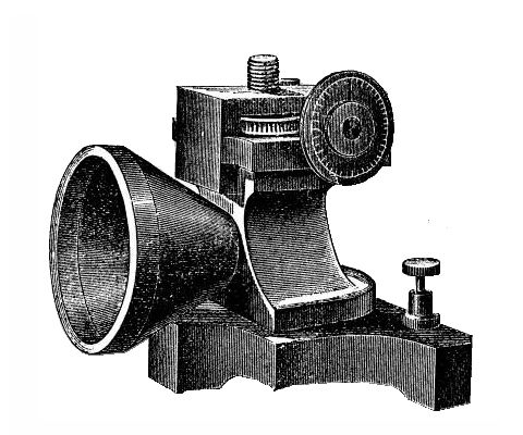
Illustration of Edison’s Tasimeter
Edison named the infrared-detecting device his “tasimeter”, and he was trying to break ground in a new scientific field in competition with the director of Pittsburgh’s Allegheny Observatory, Samuel P. Langley. Instead of letting Langley test the tasimeter’s eclipse performance alongside more proven devices such as the thermopile, Edison tried to “scoop” the competition with his solo work, and failed.
Although Langley also failed to estimate the heat coming from the solar corona with his thermopile, less than a year later he had invented the first bolometer, which is commonly used today in its most refined designs. Langley’s bolometer was so sensitive that it could detect the heat produced by a cow from a quarter of a mile away.
Although the temperature of the Sun’s corona has since been measured with bolometers, the reason why it is so hot – about 1.5 million Kelvin, considerably hotter than the Sun’s surface (5800K) – remains a theoretical problem in physics to this day.
Therefore, if you want to simulate an eclipse, or to prepare for the real thing, don’t neglect the auditory experience. Consider all possible distractions that could disrupt observations in advance, and avoid them. If you are standing near a farm in Wyoming, as the darkness approaches the sound of confused barnyard animals will reach a crescendo.
The new book American Eclipse offers a more in-depth view of the Solar Eclipse of 1878, following the trevails of Edison, planet hunter James Craig Watson, and astronomer Maria Mitchell.
Sources:
“On the Total Solar Eclipse of July 29th, 1878”, George F. Barker, Proceedings of the American Philosophical Society, Vol. 18, pp. 103-113, 1878. ( https://archive.org/details/jstor-982766 )
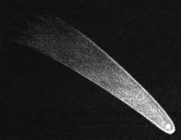
Great Comet of 1811 as drawn by William Henry Smyth
The May issue of Sky and Telescope magazine has a timely item about “Napoleon’s Comets”. The most important of these was the Great Comet of 1811, which was the brightest comet with the longest duration of brightness on record (260 days) until Comet Hale-Bopp shattered that record in 1997.
It is referred to as “Napoleon’s Comet” because of the Napoleonic Wars and the impending War of 1812, in which the United States was allied with France, Germany and Austria against Britain, Spain, Portugal, and Russia. The wars are the backdrop for the novel War and Peace by Tolstoy, and also the newly Tony-award-nominated Broadway musical Natasha, Pierre and the Great Comet of 1812 based on a small part of the novel.
The Comet of 1811 was discovered in March of that year in what is now the constellation Puppis, and it was very bright in the evening sky in September and lingered for the rest of that year. The head and coma of the comet was reported to be wider than the diameter of the Sun and it had a very long, bright tail despite not coming very close to the Earth. The Comet was held to be responsible for unusually fine vintages of French wines harvested from the Autumn 1811 grape harvest, and it is possible that Napoleon was influenced in his decision to invade Russia in June 1812 if he thought of the comet as a portent of victory.
In the US midwest, the Comet was visible during the New Madrid Earthquakes in December 1811. The Shawnee leader Tecumseh, who was born in the year of the Comet of 1769 and was named accordingly, invoked the Comet of 1811 as he built a confederacy of tribes which allied with the British in the War of 1812.
The Comet of 1811 is only mentioned on one page at the conclusion of the first half of War and Peace, but it’s misnamed the Comet of 1812. Accordingly, although the musical is titled Natasha, Pierre & the Great Comet of 1812, the Comet only appears in the finalé and is not depicted in the publicity for the production. You have to go and see it for yourself. Dave Malloy, the creator of the show, says the Comet nevertheless got into the title of the show “for cosmic epicness”.
The Broadway production this year has been nominated for 12 Tony awards, so I can’t imagine it not being talked about in planetariums.
SciDome Implementation
You can add the orbit of the Great Comet of 1811 to your SciDome by right-clicking on the Sun in Starry Night Dome Preflight and selecting “New Comet…” In the orbit specification window that pops up, enter the following values:
Name: Great Comet of 1811
Eccentricity: 0.9951250
Pericentre distance: 1.0354120
Ascending node: 143.0497000
Arg of pericentre: 65.4097000
Inclination: 106.9342000
Pericentre time: 2382768.2562000
Elements epoch: 2382760.5
And in the “Other Settings” tab, change the Diameter to 40 km and change the Absolute magnitude to 0.
“X” out of the new orbit window and confirm you want the changes to be saved. Then quit out of Starry Night properly.
If you are using Starry Night Dome version 6, the comet will be loaded on to the Renderbox when Starry Night is properly exited and will be available the next time the application is started. Because it is a user-created object, though, it will be automatically “hidden” until you uncheck it in the “Hide” column of the Find Pane. Then you can save some favourites showing the sky in the year 1811 featuring it for later playback.
If you are using Starry Night Dome 7, the comet will be saved into a file named User Planets.ssd in the Preflight folder:
C:\Users\Spitz\AppData\Local\Simulation Curriculum\Starry Night Prefs\Preflight
And that file will need to be manually ported over to the corresponding location on the Renderbox. Future versions of Starry Night Dome V7 will make this process automatic.


 Three long-awaited fulldome astrophysics apps created by Dr. David H. Bradstreet