
Aug 31, 2017 | Gravity, History, Scientific Method, Software, Solar System
 Three long-awaited fulldome astrophysics apps created by Dr. David H. Bradstreet are now available for purchase and immediate download for installation on SciDome systems. Tides, Newton’s Mountain and Epicycles are selling for $200 individually or $500 for all three.
REQUIRES WINDOWS 7 ON THE RENDERBOX COMPUTER. Multi-projector systems must be based on Scaleable – not compatible with EasyBlend.
Purchase Astrophyics Apps
These programs teach the difficult concepts of tides, orbital motion, and epicycles in unique ways on your dome. All three programs are completely controllable via an intuitive interface on your Preflight computer. In addition, Tides is controllable via SciTouch for a seamless teaching experience for your audience.
The respective At A Glance teaching guides are all available for free download if you’d like to preview what you can do with these unique Fulldome interactive programs:
Jun 12, 2017 | Fulldome Curriculum, Orbits, Planets & Moons, Scientific Method, Solar System
Volume 3 of the Fulldome Curriculum includes a lesson based on the Titius-Bode “Rule.” In this new teaching module we present the orbits predicted by the Titius-Bode relation in a historical timeline compared to the actual planetary orbits to show students why this apparent rule was important in 18th and 19th century astronomy.
The Titius-Bode “Rule” purports to describe an apparent mathematical correspondence in the sizes of the orbits of the classic planets in our Solar System. Although the idea of some kind of relationship had been hypothesized before Johann Daniel Titius and Johann Elert Bode, their publications in 1766 and 1772, respectively, brought this relation into the limelight of astronomical thought, and hence it is named after them.
The idea is that there is a mathematical relationship between each of the orbits of the classic planets. Usually it is presented in the following form:
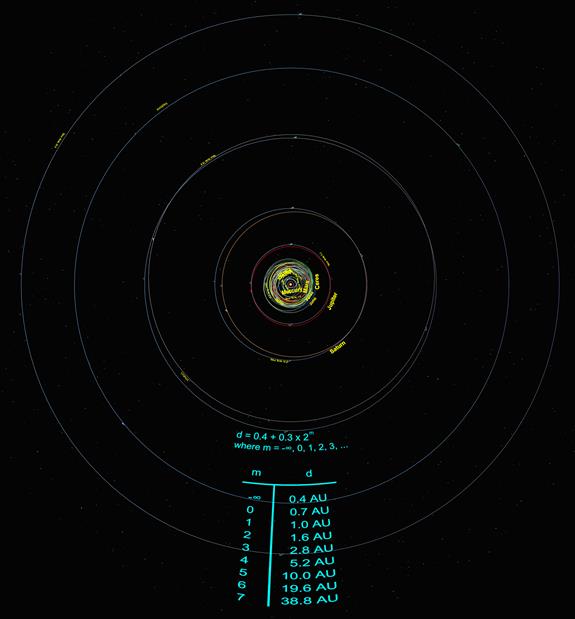
d=0.4+0.3x2m
… where m = -∞, 0, 1, 2, 3,… and d is the semi major axis of the planet in astronomical units.
Historically, this relationship was believed to be revealing something intrinsic about the positioning of the planets in the Solar System, that there might have been some type of resonance phenomenon within the formation of the planets within the solar nebula. The reason for this belief came out of the astronomical discoveries which were made subsequent to its popularization in the 18th century. To see this in its historical context, let’s set up a table the way it would have been constructed in the late 1700’s:
Interesting results, but the huge gap between Mars and Jupiter posed a real problem!
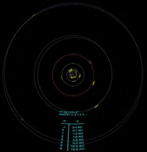
SciDome view showing Uranus’ orbit
compared to the Titius-Bode prediction
Shortly after the Titius-Bode “Law” became publicized, William Herschel in 1781 discovered a new planet, Uranus! This was a paradigm changing discovery, but what was just as incredible was that its semi major axis was calculated to be 19.2 AU, nearly doubling the size of the Solar System! Just as remarkable, the next predicted semi major axis from the Titius-Bode “Law” was 19.6 AU, only 2.1% different from the measured size!
This discovery started astronomers thinking that perhaps there was more to the Titius-Bode “Law” than they once thought, that perhaps it wasn’t coincidence but was revealing a yet undiscovered physical relationship within the Solar System. Twenty years later, on the first night of the new century, 1801, Father Giuseppe Piazzi discovered a new “planet,” later named Ceres.
What was truly remarkable about this new planet was that it’s semi major axes was eventually calculated with a new mathematical method by Carl Friedrich Gauss to be 2.8 AU, nearly exactly what the Titius-Bode “Law” had predicted for a planetary body residing in the gap between Mars and Jupiter! Of course soon thereafter many more bodies were discovered to reside within the gap, and by the 1850’s these objects were renamed asteroids.
However, the belief in the Titius-Bode “Law” was gaining new proponents, since it seemed to have predicted positions in which Solar System objects were subsequently discovered! The next predicted orbit would lie at 38.8 AU, and the search was on for yet another planet! Sure enough, Neptune was discovered with the aid of Newtonian physics in 1846, but its semi major axis was 30.1 AU, not the 38.8 AU expected from the Titius-Bode relationship.
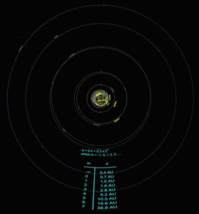
SciDome display showing the large discrepancy between Neptune’s orbit (30.1 AU) and the predicted Titius-Bode orbit of 38.8 AU
This large discrepancy led to the virtual abandonment of the Titius-Bode relationship as a physical law. However, it’s interesting to note that when Pluto was discovered in 1930 its semi major axis was determined to be 39.5 AU, very close to the previously expected distance. Of course Pluto has now been relegated to dwarf planet status because of the myriad of new objects which have been discovered in the Kuiper Belt.
The next expected semi major axis from the Titius-Bode relationship is 77.2 AU. And isn’t it interesting that Sedna’s perihelion distance is 76.1 AU, although its semi major axis is a whopping 506.8 AU!
The moral of the story seems to be that although the Titius-Bode relationship has never been convincingly proven to come from physical laws, it is noteworthy historically but also serves to perhaps warn us about jumping to conclusions even though the initial evidence may seem inviting. The Titius-Bode relationship is today such a controversial topic that Icarus, the main professional journal for presenting papers on Solar System dynamics, refuses to publish any articles on the subject!
May 30, 2017 | Eclipses, History, Scientific Method
Witnessing a total solar eclipse could change your life. Unpredicted eclipses have changed the progression of historical events. The unexpected environmental effects of a sudden darkness at midday can be very unsettling to people and animals alike.
On July 29, 1878, Thomas Edison observed the total eclipse of the Sun as part of Henry Draper’s Expedition to Rawlins, Wyoming Territory. (Although this year’s total eclipse will pass through Wyoming, the City of Rawlins will be some distance south of the total path this time.) Edison was there to test a new invention that could detect infrared light and estimate the temperature of objects remotely, and he planned to try and estimate the heat of the Sun’s corona while the solar photosphere was blocked by the Moon.
Edison’s preparations for the eclipse were not as cautious as they should have been. Because total eclipses happen close to home so very rarely (2017 is the first year that the totality has appeared in US skies since 1979), and due to the practicalities of 19th century life, most astronomers arrived at the observing site early to uncrate their heavy observing equipment and build observing shacks, and mix concrete to make steady piers. Edison arrived with a few days left before the eclipse, without time to build a protective structure, so he used the existing shelter provided by a chicken coop. On eclipse day, as the sky darkened, the bewildered chickens literally came home to roost, disrupting his observations.

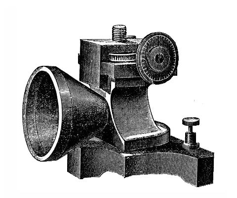
Illustration of Edison’s Tasimeter
Edison named the infrared-detecting device his “tasimeter”, and he was trying to break ground in a new scientific field in competition with the director of Pittsburgh’s Allegheny Observatory, Samuel P. Langley. Instead of letting Langley test the tasimeter’s eclipse performance alongside more proven devices such as the thermopile, Edison tried to “scoop” the competition with his solo work, and failed.
Although Langley also failed to estimate the heat coming from the solar corona with his thermopile, less than a year later he had invented the first bolometer, which is commonly used today in its most refined designs. Langley’s bolometer was so sensitive that it could detect the heat produced by a cow from a quarter of a mile away.
Although the temperature of the Sun’s corona has since been measured with bolometers, the reason why it is so hot – about 1.5 million Kelvin, considerably hotter than the Sun’s surface (5800K) – remains a theoretical problem in physics to this day.
Therefore, if you want to simulate an eclipse, or to prepare for the real thing, don’t neglect the auditory experience. Consider all possible distractions that could disrupt observations in advance, and avoid them. If you are standing near a farm in Wyoming, as the darkness approaches the sound of confused barnyard animals will reach a crescendo.
The new book American Eclipse offers a more in-depth view of the Solar Eclipse of 1878, following the trevails of Edison, planet hunter James Craig Watson, and astronomer Maria Mitchell.
Sources:
“On the Total Solar Eclipse of July 29th, 1878”, George F. Barker, Proceedings of the American Philosophical Society, Vol. 18, pp. 103-113, 1878. ( https://archive.org/details/jstor-982766 )
“Eclipse Vicissitudes: Thomas Edison and the Chickens”, J. Donald Fernie, American Scientist, Vol. 88, No. 3, May-June 2000. ( http://www.americanscientist.org/issues/pub/2000/3/eclipse-vicissitudesthomas-edison-and-the-chickens/1 )
Oct 26, 2015 | History, Orbits, Planets & Moons, Scientific Method, Software, Solar System
Our ancestors were highly intelligent people who devised ingenious methods to model what they perceived to be reality in the skies. Unfortunately, they came at many of these observations with deep-rooted prejudices and a priori (preconceived) beliefs which shackled their creativity.

Figure 1: Close up of the Ptolemaic system out to the Sun’s sphere
The prevalent, far-reaching belief was that the Earth was immovable and at the center of the universe. Of course we know this is preposterous (even to the point that there is no such thing as a center to the universe), it is still a useful exercise to challenge students to prove, without leaving the Earth or using satellites, that the Earth does indeed rotate and that it revolves about the Sun.
Another a priori assumption was that celestial bodies never stopped moving, as opposed to “earthly” objects which eventually came to a halt. So, when the planets periodically went back and forth in the sky, this was unacceptable and Apollonius of Perga came up with a “solution” that allowed the wanderers to be always moving without stopping by coupling two motions at once. The planets were not simply attached to a mystical sphere (“deferent”) but they were actually attached to a mini-sphere (“epicycle”) which rotated on the larger one.

Figure 2: Mercury’s retrograde path in the Ptolemaic system
In this way planets could move around the sky but intersperse that generally easterly motion with apparent backwards motion (retrograde) when the transparent epicycle carried the planet backwards. The ancients latched on to it and it was greatly preferred to having deferents slow down, stop, go backwards, stop, then resume their original direction.
My colleague David Steelman and I created a program called Epicycles for SciDome that illustrates the main characteristics of the Ptolemaic Geocentric Model. It helps students discover the systemics of the model which can only be explained as “it just has to be that way”. Whenever that is the reasoning, it signals a problem with the theory/model. This will become obvious as we go through this paper.
Let’s first take a close look at the bodies closest to the Earth in the geocentric model, as shown in Figure 1.
The Moon moves the fastest in the sky (and even changes shape!) so it was assumed to be closest to Earth. Placement of Mercury and Venus closer to the Earth than the Sun was problematic. The theory was based upon the idea that those that appeared to move the slowest must be farthest away from Earth. The problem is that the epicycle containing Mercury, the epicycle containing Venus, and the Sun all orbited around the Earth in one year! So their order was reluctantly agreed upon because Mercury moved fastest on it epicycle, Venus next fastest, and of course the Sun had no epicycle (because it never retrograded).

Figure 3: Venus and Mercury’s retrograde paths in the Ptolemaic system
The epicycle sizes are based on arbitrarily assumed distances from Earth. The angles had to match the size of the retrograde loops seen in the sky so, looking at Figure 1, Mercury’s epicycle is tiny compared to Venus’ because Mercury’s retrograde loop is about 52 degrees in extent whereas Venus’ is about 92 degrees! The fact that Venus is farther away than Mercury from the Earth in this model requires it to be considerably larger than one might expect, but these are to scale to create the properly sized retrograde patterns.
As time is progressed a trace can be turned on which shows the retrograding patterns of the planets. Figure 2 shows a close up of Mercury and Figure 3 that of Venus.
When I ask students if they see anything peculiar as time progresses, eventually someone notices that the centers of the epicycles of Mercury and Venus are exactly and always lined up with the line connecting the Earth and Sun (the Earth-Sun Line). What explanation would the ancients have given for this? “It just has to be this way for this model to work.” Red flag number 1 that there’s something wrong with this theory.

Figure 4: The planets beyond the Sun’s sphere
Of course we know that in the Copernican heliocentric model we don’t need epicycles to cause Mercury and Venus to wobble back and forth around the Sun because they are simply closer to the Sun than Earth and they orbit the Sun. In fact, Copernicus was the first to completely untangle the motions of Mercury and Venus from the Sun’s motion.
This confusion is one rarely-discussed reason why the Copernican heliocentric model was so appealing. It unambiguously separated the motions of Mercury and Venus and even established, for the first time, their orbital periods around the Sun (88 days and 225 days, respectively).
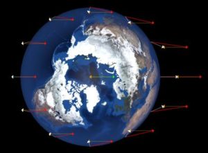
Now observe the planets beyond the Sun, as shown in Figure 4. As we advance time another strange systematic displays itself, although this one is a lot more challenging to pick out. The Earth-Sun Line is always parallel to the planet’s epicycle radius! You can easily see this in Figure 4 now that you know to look for it.
Again, the ancients noted this “coincidence” but could never explain it other than “it has to be this way for the model to work.” Another red flag has raised itself in the flawed Ptolemaic model! The basic reason for this “coincidence” is because the retrograde motion of each planet is a function of its position relative to the Earth in its own orbit. Since we’re locking down the Earth and moving the Sun, it’s the orientation of the Earth-Sun Line that is the determining factor as to when planets exhibit their retrograde motions.

Figure 5 – The retrograde paths of the planets beyond the Sun’s sphere
When the planets leave breadcrumbs (see Figure 5) their retrograding paths become obvious. Again, the model has been carefully defined to accurately recreate the width of the retrograde loops as well as their frequency.
This is a fun and thought provoking lesson for my students because it demonstrates how intelligent and clever the ancients were in mimicking celestial motions, but it also shows how preconceived notions can weigh one down and severely complicate the model. It also clearly points out that when certain “features” of a model have no other explanation than “it has to be that way for the model to work” that the model is most likely flawed or incorrect at its core. But having the Earth move was a huge paradigm shift, and it took over 1500 years to overthrow it!
Apr 20, 2015 | Fulldome Curriculum, Planets & Moons, Scientific Method, Solar System, Time
In the 17th century the speed of light was unknown, and scientists questioned whether it had a finite value. Descartes argued that if the speed of light was finite, when we looked out into space with telescopes we’d be looking into the past. That idea was so off-putting, he concluded the speed of light must be infinite.
We now know it’s not infinite. If it were, the universe couldn’t exist. Remember Einstein’s famous E=mc²: if the speed of light c was infinite, the amount of energy contained in any amount of matter would be infinite! Good luck with that…
Ole Roemer, a Danish astronomer in the 17th century, stumbled upon the speed of light during timing observations of the emergence of Jupiter’s closest Galilean moon, Io, from behind the planet’s limb. He noticed the moon’s appearances didn’t match his predicted times, and by studying them through the year realized it was ahead or behind the predicted time, depending upon how far away Jupiter was from Earth! He correctly reasoned that this variation was not due to some strange inconsistency with Io’s orbit but rather that he was observing what is now called the light-time effect.
Starry Night simulates the light time effect, so we can reproduce Roemer’s 1676 measurements of Io’s emergence from Jupiter’s limb to directly show the light time effect, and even measure the speed of light.

Figure 1: Io emerging from Jupiter’s eastern limb
Figure 1 shows Io emerging from Jupiter’s eastern limb. This view was measured by Roemer in Copenhagen on November 9, 1676. Using Starry Night’s ability to transport us anywhere in space, we can specify a direct route to Jupiter but hold the time constant.
In other words, if we could transport instantly to 0.20 AU from Jupiter (an arbitrarily distance for a nice view of the scene), what would we see? As we travel to Jupiter, we’ll see Io appear to move further and further eastward from the limb even though time has stopped and we’re traveling on a direct line to Jupiter, as shown in Figure 2.

Figure 2: Io appears farther from Jupiter as we reduce our distance
If the speed of light were infinite, when we transported to Jupiter Io would be emerging from the limb, the same view as from Copenhagen. Because the light time effect is built into Starry Night, we see Io has actually emerged significantly past the limb. In other words, on Earth we saw Io just emerging from Jupiter’s limb, but in the neighborhood of Jupiter it has already long since passed from behind the limb!
The difference occurs because of the light time effect.
We can measure the speed of light directly from these observations. We know the distance we covered in our journey from Earth (5.326 AU = 7.968 x 10⁸ km). We can now step back time and return Io back to its emerging position from Jupiter’s limb as seen from this nearby location to Jupiter. If we place Io back on Jupiter’s eastern limb by reversing time in Starry Night, it takes 44m 20s to do so, or 2660 seconds. To estimate the speed of light, we simply take the distance we traveled and divide it by the time, as follows:

Thus we obtain a value for the speed of light only 0.08% different from the actual value of 299,792 km/s!

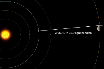
Figure 3: Line of sight from Earth to Jupiter’s limb
Steve Sanders (Eastern University Observatory Administrator) and I have created a simulation which clearly illustrates this phenomenon, as seen in the figures below. This simulation will be included in the release of Volume 3 of the Fulldome Curriculum and you can preview it on Youtube.
Figure 3 shows the line of sight from Earth to Io as it has emerged past Jupiter’s limb, the event that Roemer was measuring. We depict the event close to opposition with Jupiter (Earth’s closest approach to the planet) and the distance between the bodies is approximately 3.95 AU = 3.67 x 10⁸ million miles.
The same event is shown in Figure 4 when Earth and Jupiter are nearing conjunction (Jupiter nearing a syzygy with the Earth and Sun in between). Note that the distance separating the planets is now 5.75 AU = 5.34 x 10⁸ million miles.

Figure 4: Earth and Jupiter nearing conjunction
Roemer measured the emergence of Io as being about 15 minutes later than when this emergence occurred close to opposition and attributed the lateness (correctly) to the extra distance that the light had to travel across the Earth’s orbit.
If you assume that this tardiness is entirely due to the extra time required for light to travel the extra distance, you can estimate the speed of light as follows:

The value of the astronomical unit at that time was very crudely known, so Roemer’s value for the speed of light was not nearly this accurate, but nonetheless he demonstrated that the speed of light was finite, and its value was of this order.
We encourage SciDome operators to use the Roemer Speed of Light minilesson in Volume 1 of the Fulldome Curriculum, along with our new simulation. The discovery of the finite speed of light forever changed our view of the universe, turning our distance-shrinking telescopes into literal time machines as we explore back into our cosmic past.