Recently Spitz (thanks to Software Architect, Clint Weisbrod) implemented new guide lines in Starry Night, graphically linking the Sun and planets (see the fall 2018 Spitz Newsletter and the Copernican Method). This inspired me to consider an animated, user-controllable version depicting Kepler’s Second Law. I have already implemented static images created by Steve Sanders (Eastern University’s Observatory Administrator) for teaching Kepler’s Second Law in Volume 2 of the Spitz Fulldome Curriculum, but static images pale in comparison to animations depicting the same concept.
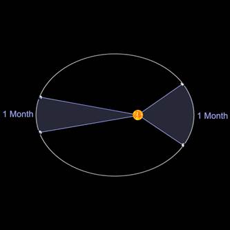
Figure 1 – Kepler’s Second Law from FDC Volume 2
Kepler’s Second Law states that a radius vector connecting a planet to the Sun will sweep out equal areas in equal intervals of time. This paradigm-shattering result enabled the understanding of how planets change velocities in an orderly and systematic fashion (they are actually conserving angular momentum, but that realization would have to wait for Newton). Historic models mimicking the changing speeds of planets were complex and impressive but completely unwieldy when it came to calculations. They were also inaccurate.
What we devised (to be included in Fulldome Curriculum Volume 4) is a new Starry Night feature allowing Kepler’s Second Law to be illustrated for bodies in the solar system (planets, moons around planets, asteroids, comets, etc.), as well as exoplanets around their parent star. The feature allows operators to make a real-time graphical version of the sweeping sections of orbits.
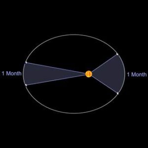
The controls for making Kepler Orbits are shown below:
The operator can enter time intervals for orbital segments (and we included a “Suggest Interval” function, which I almost always use, so beginning users have help in creating the segments). We can show individual orbital areas, and label the results.
Figure 2 – Kepler Orbit Section option dialog for Mercury
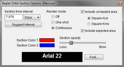
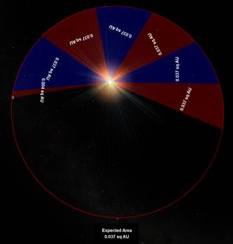
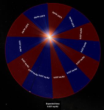
Figure 3a shows the result of running time for Mercury and Figure 3b displays the completed orbit. The numbers in each orbit segment are the numerically integrated areas of the segments, each of which is being calculated for the exact time interval set in the input box of Figure 2.
Figure 3a – Mercury beginning to draw Kepler Orbit sections in 7 day intervals
Figure 3b – Mercury completed Kepler Orbit sections in 7 day intervals
Note the Expected Area displayed at the bottom of the figures. This is the analytically calculated area for an orbital segment for Mercury given the time interval specified by the user. You may think, “Of course they are the same.” If you know anything about numerical analysis, it’s quite impressive that the numerical integration techniques implemented in this routine are accurate enough to reproduce the analytical prediction, i.e., validating Kepler’s Second Law.
We are so used to seeing equations predict outcomes that we’ve lost the astonishment of Kepler and Renaissance scientists for the precise nature of the universe, that it could be accurately modeled by mathematical equations!
Let’s take a look at this feature for Halley’s Comet. Because of the extreme eccentricity typical of comets, we’ve only displayed the perihelion passage of this body, as illustrated in Figure 4.
Figure 4 – Perihelion passage of Halley’s Comet in 1986
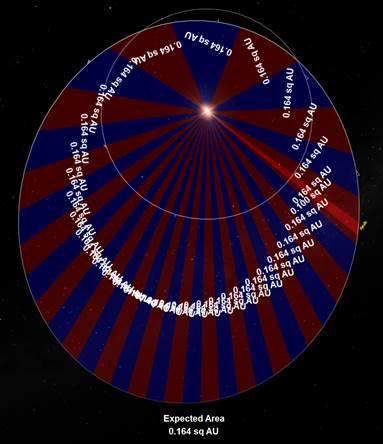
Figure 5 displays the eccentric (0.56) Venus orbit-crossing asteroid 27 Apollo around the Sun. Venus’ orbit is shown to scale.
Figure 5 – The orbit of the Venus orbit-crossing asteroid 27 Apollo
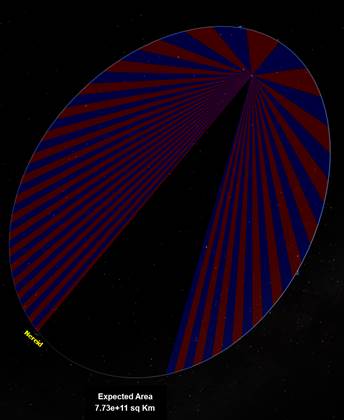
Figure 6 displays the very eccentric (0.75) orbit of Nereid, a moon of Neptune. I purposely didn’t display the numerically calculated areas to show what that looks like, i.e., to clean up the display.
Figure 6 Nereid’s orbit around Neptune, with an eccentricity of 0.75.
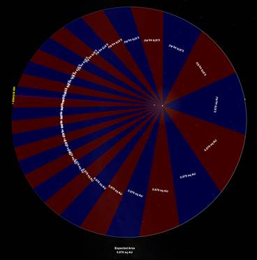
As a final example, Figure 7 displays the orbit of the exoplanet HD 87646b. It has an eccentricity of 0.500, an orbital period of 674 days and a semimajor axis of 1.580 AU.
Figure 7 – The orbit of exoplanet HD 87646b.
I sincerely hope that this upcoming new feature in SciDome excites audiences as much as it does all of us who have worked on implementing it! I also am extremely hopeful that when audiences see Kepler’s Second Law in action that they will finally be able to understand more fully what is meant by it.
Earlier this month, another “multi-messenger” announcement was made of the discovery of a new astronomical outburst by different instruments that study different parts of the universe. The first major multi-messenger astronomy discovery was announced last year after the collision of two neutron stars was observed in the nearby galaxy NGC 4993. The neutron star collision was observed first with the LIGO and Virgo gravitational wave detectors, coincident with a gamma ray burst detected by the Fermi space telescope, pinpointed with an optical telescope in South America, and followed up with different kinds of detectors.
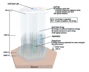
This new announcement is based on the detection of a very unusual neutrino or “ghost particle” at the IceCube Neutrino Observatory at the South Pole. This event is worth pointing out in SciDome because we have a horizon panorama that matches the horizon at the South Pole, and one or two other points that may help students understand how the sky works and what neutrinos are.
Neutrinos have been observed with detectors in both the northern and southern hemispheres of Earth, and they are created as a byproduct of various nuclear reactions. Neutrinos hardly interact with normal matter at all, and they tend to radiate outwards from their point of creation at the speed of light.
Neutrinos at rest were assumed to be massless until evidence to the otherwise shown by Art McDonald and Raymond Davis, Jr., led to them being awarded the Nobel Prize in Physics in 2015.
The interaction of neutrinos with normal matter is so weak that most neutrinos that encounter the Earth fly straight through it without hitting anything. In February 1987 when a nearby supernova popped off in the Large Magellanic Cloud, 25 neutrinos were detected at neutrino observatories in the northern hemisphere, where the Large Magellanic Cloud never rises above the horizon.
The new neutrino detection from IceCube at the South Pole was detailed enough to provide a vector back to its point of origin, somewhere within a 1.3-degree-wide circle on the sky.
The Spitz Fulldome Curriculum, included with every SciDome system, includes dozens of lessons prepared by noted astronomy educator Dr. David Bradstreet
The circle enclosed a radio source discovered in 1983, a galaxy 3.7 billion light years away with an active supermassive black hole at its core. This is one of the quasars like Dr. Bradstreet uses in his “Quasars Fulldome” show from the Fulldome Curriculum Vol. 3. Because this quasar’s jet is pointed at us, it is called a “blazar”; this term originated because the first of its type happened to be named “BL Lacertae”, and because blazars can appear brighter than normal quasars and their brightness can vary more quickly than normal quasars.
Like before, this neutrino detected from the South Pole had flown through the Earth to get to the detector. The blazar TXS 0506+056 is located at about 5 hours right ascension and +5° north of the celestial equator. Only objects south of the celestial equator are above the horizon as seen from the South Pole.
TXS 0506+056 is conveniently located in the Shield of Orion, part of the most easily recognized equatorial constellation on the sky. The blazar is labeled “MG 0509 +0541” in SciDome and is one of the quasars in Dr. Bradstreet’s “Galactocentric Distributions” minilesson.
In the part of the Fulldome Curriculum “Seasons” class that visits the South Pole, the audience may have a hard time recognizing Orion because it is upside down and its northern half, including TXS 0506+056 is below the horizon. The horizon needs to be switched off and then tilted up to bring the rest of the constellation into view to simulate a “neutrino filter”.
The prefix TXS stands for ‘Texas’, where UT-Austin astronomers set up a radio telescope array outside of Marfa for several years in the 1980s – now removed. MG stands for ‘MIT-Green Bank Observatory’.
The mass of neutrinos and other particles is calculated in electron volts, but because they are so small, only particles that have a large amount of kinetic energy are comparable to things that we can comprehend. 1 trillion electron volts (1 TeV using the prefix tera-) is comparable to the kinetic energy of a mosquito in flight. The most powerful cosmic ray ever detected had a mass of 300 quintillion electron volts, comparable to a pitched baseball.
The single neutrino detected by IceCube from TXS 0506+056 had a mass of 290 TeV. After crossing 3.7 billion light years in space, this is by far the most distant neutrino emission ever detected: the only other objects in the sky that have produced detected neutrinos have been the Sun (8 light-minutes away) and Supernova 1987A (168,000 light-years.)
(In 2012, the IceCube Collaboration detected three other high-energy neutrinos, which they named Bert, Ernie and Big Bird, but where Bert and Ernie came from is not known, and Big Bird was probably generated by the blazar PKS B1424-418 with a certainty of 95%. That’s only two sigma, which does not hold water with particle physicists who have much stricter statistical significance limits. TXS 0506+56 was much more narrowly confined.)
Because matter and energy are relative, an electron volt is equivalent to the energy exchanged by the charge of a single electron moving across an electric potential difference of one volt. The only way a neutrino can be detected is on the rare occasion when it enters a neutrino detector (like a large underground tank of heavy water or tetrachloroethylene or linear alkylbenzene or another chemical) and collides with an atomic nucleus or an electron inside the detector, emitting light that can be detected with photomultiplier tubes. IceCube is unusual because its detectors have been drilled into the Antarctic ice pack and are not suspended in water or another fluid.
Volume 3 of the Fulldome Curriculum includes a lesson based on the Titius-Bode “Rule.” In this new teaching module we present the orbits predicted by the Titius-Bode relation in a historical timeline compared to the actual planetary orbits to show students why this apparent rule was important in 18th and 19th century astronomy.
The Titius-Bode “Rule” purports to describe an apparent mathematical correspondence in the sizes of the orbits of the classic planets in our Solar System. Although the idea of some kind of relationship had been hypothesized before Johann Daniel Titius and Johann Elert Bode, their publications in 1766 and 1772, respectively, brought this relation into the limelight of astronomical thought, and hence it is named after them.
The idea is that there is a mathematical relationship between each of the orbits of the classic planets. Usually it is presented in the following form:
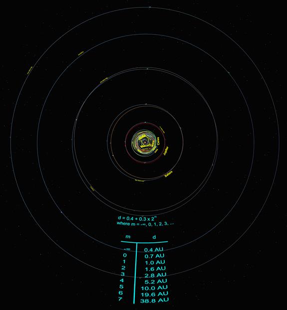
d=0.4+0.3x2m
… where m = -∞, 0, 1, 2, 3,… and d is the semi major axis of the planet in astronomical units.
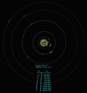
Historically, this relationship was believed to be revealing something intrinsic about the positioning of the planets in the Solar System, that there might have been some type of resonance phenomenon within the formation of the planets within the solar nebula. The reason for this belief came out of the astronomical discoveries which were made subsequent to its popularization in the 18th century. To see this in its historical context, let’s set up a table the way it would have been constructed in the late 1700’s:
Interesting results, but the huge gap between Mars and Jupiter posed a real problem!
SciDome view showing Uranus’ orbit compared to the Titius-Bode prediction
Shortly after the Titius-Bode “Law” became publicized, William Herschel in 1781 discovered a new planet, Uranus! This was a paradigm changing discovery, but what was just as incredible was that its semi major axis was calculated to be 19.2 AU, nearly doubling the size of the Solar System! Just as remarkable, the next predicted semi major axis from the Titius-Bode “Law” was 19.6 AU, only 2.1% different from the measured size!
This discovery started astronomers thinking that perhaps there was more to the Titius-Bode “Law” than they once thought, that perhaps it wasn’t coincidence but was revealing a yet undiscovered physical relationship within the Solar System. Twenty years later, on the first night of the new century, 1801, Father Giuseppe Piazzi discovered a new “planet,” later named Ceres.
What was truly remarkable about this new planet was that it’s semi major axes was eventually calculated with a new mathematical method by Carl Friedrich Gauss to be 2.8 AU, nearly exactly what the Titius-Bode “Law” had predicted for a planetary body residing in the gap between Mars and Jupiter! Of course soon thereafter many more bodies were discovered to reside within the gap, and by the 1850’s these objects were renamed asteroids.
However, the belief in the Titius-Bode “Law” was gaining new proponents, since it seemed to have predicted positions in which Solar System objects were subsequently discovered! The next predicted orbit would lie at 38.8 AU, and the search was on for yet another planet! Sure enough, Neptune was discovered with the aid of Newtonian physics in 1846, but its semi major axis was 30.1 AU, notthe 38.8 AU expected from the Titius-Bode relationship.
SciDome display showing the large discrepancy between Neptune’s orbit (30.1 AU) and the predicted Titius-Bode orbit of 38.8 AU
This large discrepancy led to the virtual abandonment of the Titius-Bode relationship as a physical law. However, it’s interesting to note that when Pluto was discovered in 1930 its semi major axis was determined to be 39.5 AU, very close to the previously expected distance. Of course Pluto has now been relegated to dwarf planet status because of the myriad of new objects which have been discovered in the Kuiper Belt.
The next expected semi major axis from the Titius-Bode relationship is 77.2 AU. And isn’t it interesting that Sedna’s perihelion distance is 76.1 AU, although its semi major axis is a whopping 506.8 AU!
The moral of the story seems to be that although the Titius-Bode relationship has never been convincingly proven to come from physical laws, it is noteworthy historically but also serves to perhaps warn us about jumping to conclusions even though the initial evidence may seem inviting. The Titius-Bode relationship is today such a controversial topic that Icarus, the main professional journal for presenting papers on Solar System dynamics, refuses to publish any articles on the subject!
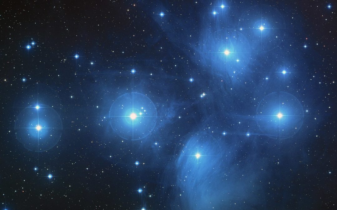
During a recent planetarium conference session, an interesting question came up about why the Pleiades is listed as M45 in Messier’s catalog. Few people know the reason for it.
Charles Messier is best known for his list of some of the best deep sky objects in the sky, and most everyone knows that he ostensibly put this list together to alert other sky watchers so that they wouldn’t mistake any of these objects for comets. Of course discovering comets was the big thing in those days because the comet was then named after the discoverer!
This reasoning begs the question as to whythe Pleiades, the bright and nearby Seven Sisters open cluster (which has been well known since antiquity), was designated as M45! No one is going to mistake this for a comet, and everyone knew of its existence! What gives?
In reality, there’s more to this mystery than just M45. Messier accidentally discovered M41 (an open cluster SW of Sirius) in 1765 – so at that time his list contained 41 objects. He decided to publish the list in 1771, but that list had 45 objects.
Note the last 4 are well-known objects, objects that had been detected by the naked eye for many centuries:
None of these objects could possibly be mistaken for a comet! Although no one knows for certain, it seems that Messier wanted to have a longer list with a more “rounded” number of objects in it than 41, hence the addition of four well-known objects for this first publication by measuring their positions himself.
My suspicion (and that of some others as well, see references) is that he wanted to have more objects in it than a well-known list published by Lacaille in 1755 which had 42 objects in it. While this is only speculation, it certainly makes sense from an egotistical point of view. After all, why else did people want to discover comets so badly?
M42 through M45 are all up in the late winter-early spring sky so markers could be placed on all four of them at once to emphasize this. This could make an interesting little side note planetarium lesson for your audiences.
Spitz is developing a Fulldome Curriculum Mini-lesson based on this idea in the future, but I thought I’d relay this interesting hypothesis beforehand in case you want to steal it for your own use.
Messier’s Nebulae and Star Clusters, Kenneth Glyn Jones (1968; 1991), p. 352
The Messier Album, John H. Mallas and Evered Kreimer (1978), pp. 1-16 (historical introduction written by Owen Gingerich, originally published in Sky and Telescope, August 1953 and October 1960)
In the 17th century the speed of light was unknown, and scientists questioned whether it had a finite value. Descartes argued that if the speed of light was finite, when we looked out into space with telescopes we’d be looking into the past. That idea was so off-putting, he concluded the speed of light must be infinite.
We now know it’s not infinite. If it were, the universe couldn’t exist. Remember Einstein’s famous E=mc²: if the speed of light c was infinite, the amount of energy contained in any amount of matter would be infinite! Good luck with that…
Ole Roemer, a Danish astronomer in the 17th century, stumbled upon the speed of light during timing observations of the emergence of Jupiter’s closest Galilean moon, Io, from behind the planet’s limb. He noticed the moon’s appearances didn’t match his predicted times, and by studying them through the year realized it was ahead or behind the predicted time, depending upon how far away Jupiter was from Earth! He correctly reasoned that this variation was not due to some strange inconsistency with Io’s orbit but rather that he was observing what is now called the light-time effect.
Starry Night simulates the light time effect, so we can reproduce Roemer’s 1676 measurements of Io’s emergence from Jupiter’s limb to directly show the light time effect, and even measure the speed of light.
Figure 1: Io emerging from Jupiter’s eastern limb
Figure 1 shows Io emerging from Jupiter’s eastern limb. This view was measured by Roemer in Copenhagen on November 9, 1676. Using Starry Night’s ability to transport us anywhere in space, we can specify a direct route to Jupiter but hold the time constant.
In other words, if we could transport instantly to 0.20 AU from Jupiter (an arbitrarily distance for a nice view of the scene), what would we see? As we travel to Jupiter, we’ll see Io appear to move further and further eastward from the limb even though time has stopped and we’re traveling on a direct line to Jupiter, as shown in Figure 2.
Figure 2: Io appears farther from Jupiter as we reduce our distance
If the speed of light were infinite, when we transported to Jupiter Io would be emerging from the limb, the same view as from Copenhagen. Because the light time effect is built into Starry Night, we see Io has actually emerged significantly past the limb. In other words, on Earth we saw Io just emerging from Jupiter’s limb, but in the neighborhood of Jupiter it has already long since passed from behind the limb!
The difference occurs because of the light time effect.
We can measure the speed of light directly from these observations. We know the distance we covered in our journey from Earth (5.326 AU = 7.968 x 10⁸ km). We can now step back time and return Io back to its emerging position from Jupiter’s limb as seen from this nearby location to Jupiter. If we place Io back on Jupiter’s eastern limb by reversing time in Starry Night, it takes 44m 20s to do so, or 2660 seconds. To estimate the speed of light, we simply take the distance we traveled and divide it by the time, as follows:
Thus we obtain a value for the speed of light only 0.08% different from the actual value of 299,792 km/s!
Figure 3: Line of sight from Earth to Jupiter’s limb
Steve Sanders (Eastern University Observatory Administrator) and I have created a simulation which clearly illustrates this phenomenon, as seen in the figures below. This simulation will be included in the release of Volume 3 of the Fulldome Curriculum and you can preview it on Youtube.
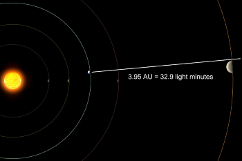
Figure 3 shows the line of sight from Earth to Io as it has emerged past Jupiter’s limb, the event that Roemer was measuring. We depict the event close to opposition with Jupiter (Earth’s closest approach to the planet) and the distance between the bodies is approximately 3.95 AU = 3.67 x 10⁸ million miles.
The same event is shown in Figure 4 when Earth and Jupiter are nearing conjunction (Jupiter nearing a syzygy with the Earth and Sun in between). Note that the distance separating the planets is now 5.75 AU = 5.34 x 10⁸ million miles.
Figure 4: Earth and Jupiter nearing conjunction
Roemer measured the emergence of Io as being about 15 minutes later than when this emergence occurred close to opposition and attributed the lateness (correctly) to the extra distance that the light had to travel across the Earth’s orbit.
If you assume that this tardiness is entirely due to the extra time required for light to travel the extra distance, you can estimate the speed of light as follows:
The value of the astronomical unit at that time was very crudely known, so Roemer’s value for the speed of light was not nearly this accurate, but nonetheless he demonstrated that the speed of light was finite, and its value was of this order.
We encourage SciDome operators to use the Roemer Speed of Light minilesson in Volume 1 of the Fulldome Curriculum, along with our new simulation. The discovery of the finite speed of light forever changed our view of the universe, turning our distance-shrinking telescopes into literal time machines as we explore back into our cosmic past.
Figure 1: Page from the original printing of Sidereus Nunicius showing Galileo’s sketches of the Medicean Moons
In many of our astronomy classes, we discuss the importance of Galileo’s first telescopic observations in eventually overthrowing the Ptolemaic geocentric system. His first observations were relayed to the public in his short book Sidereus Nuncius, which is Latin for The Starry Messenger (or arguably, The Starry Message). In it he relates his observations of the Moon, the myriad of new stars he observed (with sketches of the Pleiades and Praesepe regions), and the Moons of Jupiter.
He originally called these the Medicean Stars, a call out to his potential benefactors, the four Medici brothers (the book itself was dedicated to one of them who had been a former pupil). Seeking for funds for your science… things really haven’t changed very much in 400 years…
With Starry Night, SciDome can easily reproduce the date and situations of Galileo’s observations. Others have done this in the past, and I refer you to the excellent article by Enrico Bernieri called “Learning from Galileo’s Errors” published in the Journal of the British Astronomical Association, 122, 3 (2012) which goes through his observations in detail and discusses the errors which Galileo made.
I also highly recommend the Wikipedia article on Sidereus Nuncius as an excellent starting point in building your background information on Galileo’s first telescopic observations. In addition, Ernie Wright has graphically reproduced Galileo’s observations and placed them online in an excellent web presentation.
With the incredible talent of Steve Sanders (Eastern University Observatory Administrator), I have created a minilesson for Volume 3 of the Fulldome Curriculum which reproduces all of Galileo’s published observations of the Medicean moons.
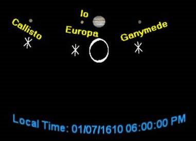
Figure 2: SciDome presentation of Galileo’s first Jupiter observations from January 7, 1610 from Padua, Italy.
Using Padua, Italy as our observation location and the approximate times given for each observation in Sidereus Nuncius, we begin with the close-up view of Jupiter on the dome as seen on January 7, 1610 at approximately 6 PM local time. Next we place a slide of the view as drawn by Galileo in Sidereus Nuncius below the view to show just how accurate Galileo was in his sketches. The labels of the Galilean moons are then displayed.
Note that although all four moons presented themselves, Io and Europa were too close together to be resolved by Galileo’s homemade 20X telescope which suffered also from chromatic and spherical aberration. This is an important fact to remember, because essentially all of the “errors” which we will find in comparing his sketches to the actual viewing circumstances were because of his lack of resolution.
We proceed by advancing time in Starry Night so that the audience can watch the dance of the moons around Jupiter and stop at the next observations of Jupiter as recorded by Galileo, on January 8, 1610. Then his sketch of this configuration is displayed, and again we note the accuracy of his rough sketches.
The minilesson continues in this fashion, showing the moons moving from date to date and then presenting 21 successive sketches by Galileo as presented in Sidereus Nuncius. Galileo concluded after four nights of observations that these tiny “stars” were indeed most likely satellites of Jupiter, which was of momentous importance because it was the first time that moons had been discovered around another body.
It also indicated that a planet could move and moons “stay up with it” despite its motion, an Aristotelian argument once offered to discount that the Earth could be moving because, if it did, how could the Moon know enough to keep up with it? Obviously Jupiter had at least four moons and they had no problem staying with it!
I have found that going through many of these configurations with my students greatly enhances their appreciation of Galileo and the great discoveries that he made despite the limitations of his equipment. Presenting this minilesson engages students in the realization that Galileo was both an excellent and honest observer as well as a genius. His observations helped to lead to the downfall of the geocentric universe and the eventual acceptance of the heliocentric model