Recently Spitz (thanks to Software Architect, Clint Weisbrod) implemented new guide lines in Starry Night, graphically linking the Sun and planets (see the fall 2018 Spitz Newsletter and the Copernican Method). This inspired me to consider an animated, user-controllable version depicting Kepler’s Second Law. I have already implemented static images created by Steve Sanders (Eastern University’s Observatory Administrator) for teaching Kepler’s Second Law in Volume 2 of the Spitz Fulldome Curriculum, but static images pale in comparison to animations depicting the same concept.
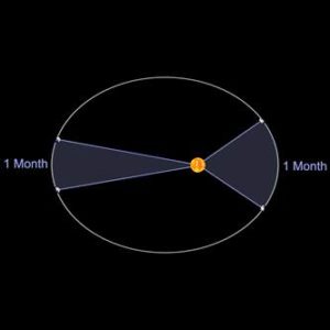
Figure 1 – Kepler’s Second Law from FDC Volume 2
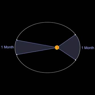
Kepler’s Second Law states that a radius vector connecting a planet to the Sun will sweep out equal areas in equal intervals of time. This paradigm-shattering result enabled the understanding of how planets change velocities in an orderly and systematic fashion (they are actually conserving angular momentum, but that realization would have to wait for Newton). Historic models mimicking the changing speeds of planets were complex and impressive but completely unwieldy when it came to calculations. They were also inaccurate.
What we devised (to be included in Fulldome Curriculum Volume 4) is a new Starry Night feature allowing Kepler’s Second Law to be illustrated for bodies in the solar system (planets, moons around planets, asteroids, comets, etc.), as well as exoplanets around their parent star. The feature allows operators to make a real-time graphical version of the sweeping sections of orbits.
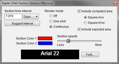
The controls for making Kepler Orbits are shown below:
The operator can enter time intervals for orbital segments (and we included a “Suggest Interval” function, which I almost always use, so beginning users have help in creating the segments). We can show individual orbital areas, and label the results.
Figure 2 – Kepler Orbit Section option dialog for Mercury
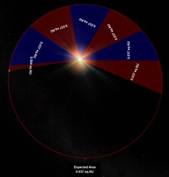
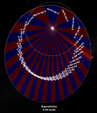
Figure 3a shows the result of running time for Mercury and Figure 3b displays the completed orbit. The numbers in each orbit segment are the numerically integrated areas of the segments, each of which is being calculated for the exact time interval set in the input box of Figure 2.
Figure 3a – Mercury beginning to draw Kepler Orbit sections in 7 day intervals
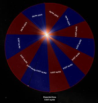
Figure 3b – Mercury completed Kepler Orbit sections in 7 day intervals
Note the Expected Area displayed at the bottom of the figures. This is the analytically calculated area for an orbital segment for Mercury given the time interval specified by the user. You may think, “Of course they are the same.” If you know anything about numerical analysis, it’s quite impressive that the numerical integration techniques implemented in this routine are accurate enough to reproduce the analytical prediction, i.e., validating Kepler’s Second Law.
We are so used to seeing equations predict outcomes that we’ve lost the astonishment of Kepler and Renaissance scientists for the precise nature of the universe, that it could be accurately modeled by mathematical equations!
Let’s take a look at this feature for Halley’s Comet. Because of the extreme eccentricity typical of comets, we’ve only displayed the perihelion passage of this body, as illustrated in Figure 4.
Figure 4 – Perihelion passage of Halley’s Comet in 1986
Figure 5 displays the eccentric (0.56) Venus orbit-crossing asteroid 27 Apollo around the Sun. Venus’ orbit is shown to scale.
Figure 5 – The orbit of the Venus orbit-crossing asteroid 27 Apollo
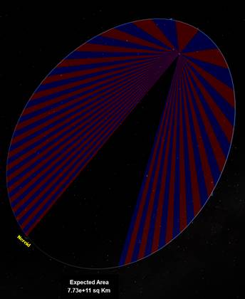
Figure 6 displays the very eccentric (0.75) orbit of Nereid, a moon of Neptune. I purposely didn’t display the numerically calculated areas to show what that looks like, i.e., to clean up the display.
Figure 6 Nereid’s orbit around Neptune, with an eccentricity of 0.75.
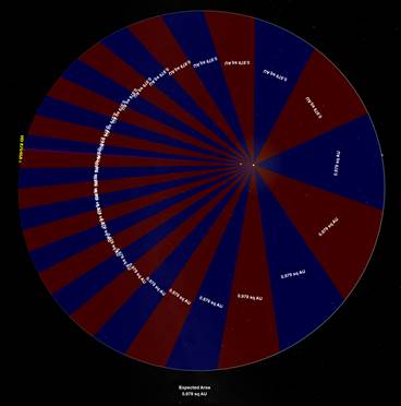
As a final example, Figure 7 displays the orbit of the exoplanet HD 87646b. It has an eccentricity of 0.500, an orbital period of 674 days and a semimajor axis of 1.580 AU.
Figure 7 – The orbit of exoplanet HD 87646b.
I sincerely hope that this upcoming new feature in SciDome excites audiences as much as it does all of us who have worked on implementing it! I also am extremely hopeful that when audiences see Kepler’s Second Law in action that they will finally be able to understand more fully what is meant by it.
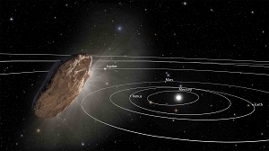
By now I hope you’re heard about the interstellar interloper that’s been passing through the inner solar system recently. This asteroid, which has been named ‘Oumuamua, is the first-ever discovered object that has been observed coming into the solar system from elsewhere in the Milky Way that is larger than tiny bits of dust.
There are several known instances of objects being “ejected” out of our solar system, so periodically there should be a chance to see a passing object that has been “ejected” from some other solar system passing by us. But only objects that pass close to the Sun or those that cast their own light are bright enough to be seen.
‘Oumuamua (NASA artist’s impression)
‘Oumuamua was discovered on Oct. 19th when it was already more than a month past its closest point to the Sun. It’s only about 300 feet across, and it was close enough to Earth to be seen for a short while.
Objects passing through the solar system that aren’t gravitationally bound to the Sun must be moving very quickly, although all paths are bent around their closest point to the Sun. The eccentricity of an elliptical orbit around the Sun is represented in the mathematical elements of the orbit by a number between zero and 1. The eccentricity of an object that is going too fast to be captured by the Sun has a value between 1 and infinity. The value in this case is about 1.2, and the object’s velocity entering the solar system was about 59,000 mph. It was probably ejected from another star many light years away and millions of years ago, although it is from the “disk” of the Milky Way and not the more exotic “halo”. A “halo” object would probably be moving faster.
‘Oumuamua’s orbit can be simulated in Starry Night Dome. The orbital elements are a little on the uncertain side because of the short duration of observations between discovery and it zipping out of range. And the effect of the over-unity eccentricity appears to “break” the position of the object during times before February 2016 or after March 2019. But the 3 years when it’s at its closest point to the Sun are replicated pretty well.
To add ‘Oumuamua to SciDome Version 7, right-click on the Sun in Starry Night Preflight and select ‘New Asteroid…’ and enter the following values in the details window that pops up, using the ‘Pericentric’ method instead of ‘Near-Circular.’ Also pick an appropriate name in the ‘Untitled’ field.
Once you close this details window and “keep” the new object, and quit SciDome properly, the new object will be written to a file called “User Planets.ssd”. You need to copy this file from its location on Preflight to the Renderbox for it to be “live” on both computers.
c:\Users\Spitz\AppData\Local\Simulation Curriculum\Starry Night Prefs\Preflight\User Planets.ssd
This file needs to be copied and installed on the Renderbox at the comparable folder location:
c:\Users\Spitz\AppData\Local\Simulation Curriculum\Starry Night Prefs\Renderbox\User Planets.ssd
Please contact me if you need a little extra guidance on making this work. After this is done, the object should be “live” in Starry Night on the dome during the current “Now”.
You can also fly out to the object and watch the planets and the Sun fly by as its lumpy asteroid shape zooms past. I would recommend one special piece of orientation for objects like this. During SciDome training, one of the choices we emphasize when looking at a solar system object from above is that you can “Rotate With” or “Hover Over” the planet or moon below. If you “Rotate With” while looking down at the United States, and speed up time, the Earth won’t appear to rotate, you can see successive nightfalls and daybreaks over North America, and the background stars will rotate around in the background. If you “Hover Over”, as time passes North America will rotate away to the east, Asia will appear out of the west and the fixed stars won’t move. The Sun Angle won’t change much either.
There is a third option in the dropdown menu that allows you to choose “Rotate With” or “Hover Over”, which is very much like “Hover Over” but not quite. It’s called “Follow in Orbit.” The small difference between “Hover Over” and “Follow in Orbit” is that “Follow in Orbit” will maintain the phase of illumination by the Sun as the planet orbits the Sun, and the fixed stars will slowly sweep by although the Sun Angle won’t change as time passes. “Hover Over” is completely inertial – as the planet orbits the Sun, the phase of the Sun Angle will slowly change and only the fixed stars will stay fixed.
We don’t always drill down far enough to distinguish between “Hover Over” and “Follow in Orbit” because it takes more than a month of time flow to accumulate a 30° difference between the two. But in the case of ‘Oumuamua, because its position with respect to the Sun changes so quickly, you might want a way to keep the Sun Angle constant so the source of illumination won’t rotate away from your point of view and you “lose the light”. “Follow in Orbit” is a useful orientation choice for an object like this.
A little bit of hay has been made of the way the incoming path of ‘Oumuamua leads back towards the constellation Lyra. This can also be simulated in Starry Night. The brightest star in Lyra is Vega, which was the fictional location of the first extraterrestrial signals in the Carl Sagan novel Contact. Sagan may have picked Vega to use in his book because it has been known for some time that the motion of the Sun and the solar system through the Milky Way is in the general direction of that star.
The great American/Canadian astronomer Simon Newcomb wrote in Elements of Astronomy – a book Sagan would have known – “The motion of our solar system toward the constellation Lyra is one of the most wonderful conclusions of modern astronomy.” However, as we move in the direction of that constellation, Lyra and the other stars in it have their own movements that will scramble them all out in other directions as time passes.
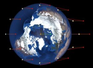
The proper motions of the stars can also be turned on in Starry Night as a series of artificial lines, and simulated back and forth through a couple of hundred thousand years of movement centered on the present if you switch to a “Stationary Location.” These proper motions may appear random, but if you highlight some of the closest and most well-known nearby stars, you can track them moving away from or toward the direction of Lyra as time passes forward or backward with some coherence.
On August 17th, the Laser Interferometer Gravitational-Wave Observatory, or “LIGO”, detected gravity waves produced by the merger of two neutron stars. There are lots of good takes on this story, and it’s important that we keep retelling it in interesting ways. This entry briefly summarizes the observations of the event, while focusing in on a couple of ways that a SciDome planetarium show about this could be exciting for an educational audience.
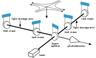
Basic components of a gravitational wave detector
A neutron star is the typical remnant left behind after a supernova explosion. Specifically, this is the kind of supernova that overtakes a massive star at the end of its lifespan, when heavy elements have accumulated at its core. Massive stars that go supernova tend to have short lifespans on the cosmic scale, only a few million years.
In a supernova, the outer layers of the star collapse onto the core, compress it, and rebound outwards in an explosion. The core is left behind, but the pressure of the infalling layers squeeze it to the point that normal matter made up of atoms can no longer exist. It is squeezed so tight that orbiting electrons and core protons violate the Pauli Exclusion Principle and combine into neutrons that have no net charge.
A neutron star is a small but extremely massive object made up of this “neutron-degenerate matter” that has no protons or electrons, with no space in between the nuclei. “Neutronium” is extremely dense, so that a teaspoon full of it would weigh two billion tonnes. The diameter of the neutron star is only a few miles.
The type of supernova that can create a neutron star tends to occur in a given galaxy roughly once per century. Neutron stars that rotate can be observed in radio waves as “pulsars”. Due to the law conservation of angular momentum on a rapidly collapsing massive object, pulsars tend to rotate extremely quickly.
The Spitz Fulldome Curriculum, included with every SciDome system, includes dozens of lessons prepared by noted astronomy educator Dr. David Bradstreet
You can review the lesson plan for the Fulldome Curriculum minilesson in your SciDome named “Galactocentric Distributions”, which has a step that highlights the locations of supernova remnants like pulsars. That ATM-4 lesson uses the Starry Night database “Supernova Remnants” which can also be toggled on and off manually.
Although neutron stars are rare (one such may be created in a galaxy of 100 billion stars after an interval of 100 years), it is possible for two pulsars to be observed orbiting each other. Since they were first observed in 1967, hundreds of pulsars have been observed in the Milky Way, and there is also a suspected population of neutron stars that can’t be observed. So far there are two known binary pulsars in the Milky Way.
Until LIGO was completed in 2002 and then upgraded in 2015, the only method of observing the effects of gravitational waves was to use a radio telescope to time the regular pulses of a binary pulsar and measure its rate of slowing. Einstein’s general theory of relativity describes gravity as a warping of space/time around massive objects. As a pair of pulsars orbit each other, some of their rotational energy is carried away by the propagation of gravitational waves. The first known binary pulsar has an orbital period of about 7 hours, and the timing of its pulses has revealed a small orbital contraction. That pair may take 300 million years to spin together.
Since LIGO was upgraded in 2015, it has started to discover gravitational wave events caused by black holes merging. Mergers of stellar-mass black holes are somewhat common in the deep cores of galaxies and maybe some other places in the universe, but so far no black hole mergers have been observed by LIGO with enough accuracy to find their host galaxies.
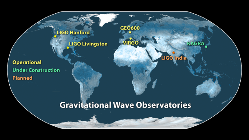
The two stations of LIGO are located in eastern Washington state and in rural Louisiana. The sensitivity of the system has recently been improved through collaboration with the European gravitational wave observatory Virgo, located outside Pisa, Italy. These locations can be visited in SciDome with The Layered Earth.
The August 17th event that’s now in the news (GW170817) was the collision of a pair of neutron stars in another galaxy. It is notable because it’s the first observed neutron star collision, and because its optical component was found thanks to triangulation between gravitational wave observatories and gamma-ray observatories.
One aspect of the breaking nature of the story is that although the news was embargoed from distribution until this week, rumors have been circulating about it since the day it happened, a few days before the total solar eclipse in August. Now that the papers have been published, notably B.P. Abbott et al. in Physical Review Letters, the scale of the collaboration becomes apparent. There are so many co-authors on these papers that it has been guesstimated that 15% of all professional astronomers are being cited. No wonder it was difficult for them to keep a secret!
The rapid outburst and the quick dimming of the object was less impressive than a supernova – maybe only a tenth as bright as a supernova, so the name “kilonova” has been proposed to distinguish this kind of an event from a supernova.
https://www.youtube.com/watch?v=nziW8fywwmg
ESO animation: Zooming in on the NGC 4993 kilonova
The host galaxy is also very close to us. One of my other hats apart from Spitz is as a supernova hunter. I’ve co-discovered ten supernovae by searching through images of external galaxies, and although it is not atypical for one or even two supernovae per year to turn up in galaxies that are less than ten million light years away, I have never found one that was closer than 215 million light years. The host galaxy, NGC 4993, is only about 120 million light years away.
NGC 4993 is so close that it was observed visually in the late 18th Century, before photography was invented, with an 18-inch reflecting telescope with a speculum metal mirror. The greatest father-and-son team of astronomers in history – William and John Herschel – found it 45 years apart.
Did I mention that neutron star collisions are rare? A given galaxy may only host a binary neutron star collision once per 100,000 years, and there are only on the order of 100,000 galaxies in the volume with radius 120 million light years.
You can look up NGC 4993 in Starry Night and dial up the location and the date of its discovery: Slough, England on March 26th, 1789. This galaxy isn’t easy to see from so far north. It only gets 16° above the southern horizon as seen from Slough.
You can also dial up the discovery date of the gravitational wave event – August 17th of this year. One of the points that’s been made is that in August, NGC 4993 sets a couple of hours after the Sun, and is not easy to find in the short time available after sunset. By the time of this week’s announcement, NGC 4993 has gone behind the Sun and no new observations can be made by anybody until it returns in the predawn sky. If the gravitational waves event had happened two months later, the source of GW170817 would not have been found.
You can also fly out to the host galaxy to observe it in three dimensions with Starry Night. The name NGC 4993 is not “flyable”, so we have to type in the name that is attached to this galaxy in one of the newer catalogs that renders it as a 3D object. In the search field, type in:
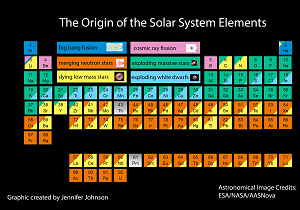
The phrase “We are star stuff” has been a part of the astronomer’s public outreach lexicon for many years, since Carl Sagan. We know how to point out that all the heavy elements that make up solid matter on Earth were fused out of lighter elements in the cores of stars, and that iron and everything heavier than it was produced by supernova explosions. It’s now time to re-invent the part of this expression that deals with a lot of those heavy elements.
The neutron star collision in NGC 4993 seems to have produced more than 10 Earth masses of gold, platinum and other precious metals. Dr. Jennifer Johnson from The Ohio State University, a SciDome user, posted a Periodic Table of the Elements on her blog that has been broken down to highlight which elements can be generated by supernovae, colliding neutron stars, etc.
Three long-awaited fulldome astrophysics apps created by Dr. David H. Bradstreet are now available for purchase and immediate download for installation on SciDome systems. Tides, Newton’s Mountain and Epicycles are selling for $200 individually or $500 for all three.
REQUIRES WINDOWS 7 ON THE RENDERBOX COMPUTER. Multi-projector systems must be based on Scaleable – not compatible with EasyBlend.
These programs teach the difficult concepts of tides, orbital motion, and epicycles in unique ways on your dome. All three programs are completely controllable via an intuitive interface on your Preflight computer. In addition, Tides is controllable via SciTouch for a seamless teaching experience for your audience.
The respective At A Glance teaching guides are all available for free download if you’d like to preview what you can do with these unique Fulldome interactive programs:
48 years ago last week Apollo 11 landed on the Moon. There is another anniversary last week that seems appropriate to mention at this point: On July 20th of 1925 the greatest scene in American legal history took place, and it was an astronomy lesson.
You’re probably familiar with the play Inherit the Wind, which was based on the Scopes Monkey Trial. In the summer of 1925, more specifically on July 20th, on the courthouse lawn in Dayton, TN, Clarence Darrow had William Jennings Bryan on the witness stand to respectively challenge and defend the state’s Butler Act that prohibited public school teachers from denying the Biblical account of the origin of humanity.
Darrow and Bryan were agreed on the terms of the Earth being a sphere, and that the Earth orbits around the Sun and not the other way round. Therefore it was necessary for them to interpret the biblical passages that seemed to indicate that the Earth was flat and that the Sun stopped at midday for Joshua.
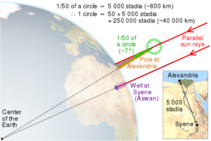
Illustration of Erastothenes’ method by CMG Lee. CC BY-SA 4.0
That the Earth was round, and that the Earth was turning and the Sun was at the axis of the solar system was not difficult to accept in 1925. People were familiar with Eratosthenes’ 3rd-Century-BC experiment in Egypt to estimate the circumference of the Earth (252,000 stadia.) They were also familiar with the great American novelist Washington Irving’s biography of Christopher Columbus, which laid out Columbus’ theory of the roundness of the Earth and his discovery of America obstructing the route to India.
That the Earth was round was also not difficult to accept in the 1480s when Columbus solicited the crowned heads of Europe to fund his voyage to India. It’s just a simplification of Washington Irving’s biography of Columbus to say that Columbus was trying to prove that the Earth was round and that his opposites held that it was flat. In the 4th chapter of the biography, the author puts Columbus in front of the School of Salamanca where he is criticized for the way he contradicts classical dogma from Saint Augustine in the 4th Century AD concerning the “Doctrine of Antipodes“.
In modernity, the antipodes are the geographic point opposite one’s position on the globe, but these medieval Antipodes were the mythical people supposed to inhabit the southern hemisphere who walked upside down (antipode meaning “reversed feet.”) but Saint Augustine did not dispute that the Earth was round:
“As to the fable that there are Antipodes, that is to say, men on the opposite side of the earth, where the sun rises when it sets to us, that is on no ground credible. And, indeed, it is not affirmed that this has been learned by historical knowledge, but by scientific conjecture, on the ground that the earth is suspended within the concavity of the sky, and that it has as much room on the one side of it as on the other: hence they say that the part which is beneath must also be inhabited. But they do not remark that, although it be supposed or scientifically demonstrated that the world is of a round and spherical form, yet it does not follow that the other side of the earth is bare of water; nor even, though it be bare, does it immediately follow that it is peopled.”
Columbus’ critics in the Inquisition, if any, subscribed to dogma that the Earth was round but that human civilization was limited to the temperate zone of the northern hemisphere by the Torrid Zone at the equator. That there was a corresponding southern temperate zone in the southern hemisphere, but that humans created in Genesis could not exist there because the Garden of Eden was in the north and the Torrid Zone was impassable or nearly so. That navigation to get there wasn’t easy because there was no North Star in the south, and the Doldrum Belt made headway under sail to the opposite end of the Earth impossible. The 1st-Century-BC Roman writer Cicero had written about the impassable Torrid Zone in an item called the Dream of Scipio, which is a good basis for an old-timey planetarium show in itself.
“Moreover you see that this earth is girdled and surrounded by certain belts, as it were; of which two, the most remote from each other, and which rest upon the poles of the heaven at either end, have become rigid with frost; while that one in the middle, which is also the largest, is scorched by the burning heat of the sun. Two are habitable; of these, that one in the South—men standing in which have their feet planted right opposite to yours—has no connection with your race: moreover this other, in the Northern hemisphere which you inhabit, see in how small a measure it concerns you! For all the earth, which you inhabit, being narrow in the direction of the poles, broader East and West, is a kind of little island surrounded by the waters of that sea, which you on earth call the Atlantic, the Great Sea, the Ocean; and yet though it has such a grand name, see how small it really is!”
It is true that Columbus was trying to sail around the world to reach India, and that he had underestimated the circumference of the Earth due to a conversion error from Eratosthenes: by the 15th Century, the value of 252,000 stadia was remembered, but the value of a stadion was uncertain, and Columbus used the wrong value. Therefore the Earth seemed smaller, and globes of the Earth from that period show the East Indies on the western edge of the Atlantic Ocean.
Columbus was convinced that the Torrid Zone was not a barrier to travel. Earlier in his career he had sailed to West Africa, almost to the Equator. The first European transit of the Cape of Good Hope (which is in the southern temperate zone) into the Indian Ocean was by the Portuguese navigator Bartolomeu Dias in 1488, two years after Columbus’s first unsuccessful examination at Salamanca.
This 1492 globe of the Earth is under a Creative Commons licence, so feel free to demonstrate it via its own API. It could be converted and wrapped around the Earth in Starry Night, but I don’t feel ready make the final product available for SciDome at this time due to the rights.
However, there are lots of ways to use SciDome to demonstrate that the Earth is round. The upcoming total solar eclipse is one event that is not easy for flat-earth believers to explain, when its occurrence is so accurately predicted with established science. Performing Eratosthenes’ experiment in SciDome is not difficult, by displaying the sky above his two observing stations in Alexandria and Aswan at local noon on June 21st with the Local Meridian switched on with graduations.
Now that we have established that the roundness of the Earth was accepted by both sides in the 1925 Scopes Trial, and that the roundness of the Earth was accepted by both Columbus and his critics (admitting serious gaps in the knowledge of both sides) and by the ancient Greeks, I hope that we can help elevate current concerns about the Earth being flat. I understand that a large billboard was recently used in suburban Philadelphia next to the freeway to state “Research Flat Earth”. And when we argue against modern flat-earth believers, we should not compare their belief to Columbus’s critics, and commit another simplification of the actual story.
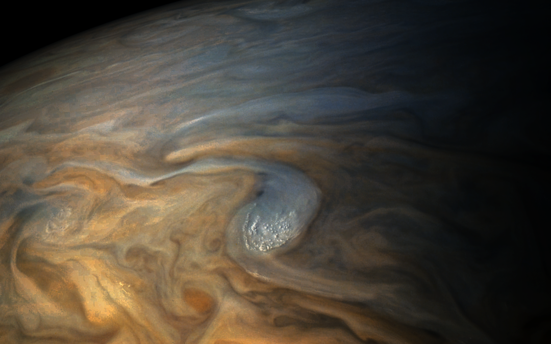
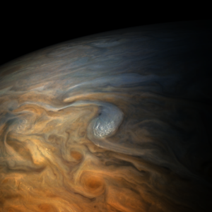
One of the astronomical highlights of last week was the pictures returned by the Juno spacecraft orbiting Jupiter when it zipped over the Great Red Spot at an extremely low altitude (8000 km.) Although the JunoCam camera on this mission was an afterthought for public outreach purposes and not a research experiment, the camera has returned some data that can be amazing when processed, and shows no signs of stopping yet, despite Jupiter’s harsh radiation environment.
To simulate this mission in Starry Night Version 7 on a Spitz SciDome planetarium, a couple of changes need to be made, even with recent updates. But with those changes made, you can simulate this flypast in Starry Night, and also think about using some of the real camera images from Juno on your dome as slides with ATM-4.
Firstly, we need to update the Space Missions file Juno.xyz. Starry Night V7 may already have a version of the mission path, but that is the *planned* mission. An anomaly in Juno’s rocket engine led to a revised mission plan with a different path. The original path does not include a periapsis over the Great Red Spot on the date in question, July 10th. To update the mission path, download this zipped folder, unzip it, and move the contained file Juno.xyz to the following location:
C:\ProgramData\Simulation Curriculum\Starry Night Prefs\Sky Data\Space Missions\Juno.xyz
This change is only made in one networked location to affect both computers, to avoid tediously installing it on Preflight and Renderbox in two steps. Files added to the “ProgramData” Sky Data folder will override files with the same names added to the old-fashioned Sky Data folder in the folder “Program Files (x86)”. The “ProgramData” structure exists so that V7 users no longer need to tediously make changes to Program Files on either computer.
Secondly, the position of the Great Red Spot needs to be updated. Jupiter is not a solid body, and the Great Red Spot has a tendency to drift, and its drift rate has a tendency to change, generating an accumulating error. So it’s not practical to just use the GRS as the index for the fixed period of rotation of Jupiter that is mapped out by the surface texture in Starry Night. The value of the drift is currently about +5° per month, and the current value of the drift is about 271° in Jupiter System II longitude. (Last week I was using a value of 269° and that also came out pretty good: 269° represents the value during the Juno encounter.)
To edit the value in Starry Night V7 for SciDome, locate the following file and open it using Wordpad (not Notepad:)
C:\Program Files (x86)\Starry Night Preflight\Sky Data\JupiterGRS.txt
You may recognize that the code inside is a little odd: Double slashes in odd places. If you are familiar with the coding, these slashes take on added significance. They should each represent the beginning of a new line of code that should be ignored by the program.
The only part of the file that is read by the program is the line that does not begin with two slashes. Please edit the file if necessary so the text is as follows, and the value is updated:
// Enter the mean longitude of the Great Red Spot on the following line. Visit // the Starry Night Pro website at http://www.starrynightpro.com to get the // latest value. 269.0
Then save the file into the ProgramData folder as follows, in a single step:
C:\ProgramData\Simulation Curriculum\Starry Night Prefs\Sky Data\JupiterGRS.txt
Once again, saving in this location means it’s not necessary to save changes on the other computer as well.
Artist’s rendering of the Juno spacecraft.
There is a 3D model of the Juno spacecraft in SciDome version 7, so you ought to be able to simulate its swooping down on the Great Red Spot in different ways: A long view of Jupiter with the Juno “Mission Path” turned on and the spacecraft labelled as a dot, or also flying alongside the spacecraft 3D model as the GRS looms on the limb of Jupiter overhead.
If you are using Starry Night Version 6 for Scidome, you can still place the attached Juno.xyz in the Space Missions folder of the original Sky Data folder on both computers and chart the updated path, but there is no 3D model of the spacecraft available. There is a separate 3D model that represents the asteroid (3) Juno, and they could get mixed up.
Because the GRS will continue to drift, you may wish to return to make subsequent edits to JupiterGRS.txt. The drift currently accumulates +5° per month, but because the drift rate can change, I recommend doing one of two things:
1) Now that you have the Juno simulation of what will probably be the best and closest images of the Great Red Spot for our lifetime, don’t make any further changes to the GRS value. Further edits to the drifting value will start to “break” the position of the GRS during the Juno flyby on July 10th, if you have built an ATM-4 automation out of it.
2) Continue to update the GRS position to represent reality based on observations, not predictions to avoid accumulating drift error. The current System II longitude of the GRS is kept up to date in a couple of places on the Internet, such as CalSky.
It is possible that Juno will have another encounter with the Great Red Spot on one of its remaining orbits, but the period of its orbit around Jupiter is 53 days. In multiples of 53 days the GRS position value will change by multiples of 9°, with some accumulation of error, and the orbital period of the spacecraft is not an integer multiple of the rotation period of Jupiter. Let’s wait and see.

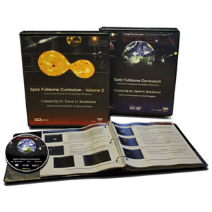

 Three long-awaited fulldome astrophysics apps created by Dr. David H. Bradstreet