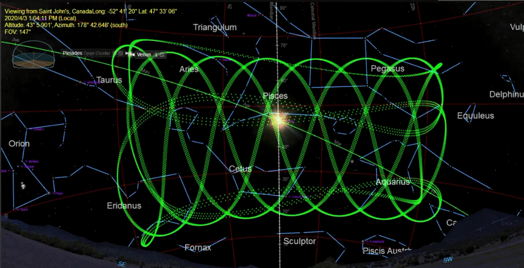
There is an upcoming event in the evening sky that is worth notifying your colleagues about on social media this week. Venus is going to pass in front of the Pleiades star cluster on Friday, April 3rd. The neat thing about it is that this happens every 8 years, to the day. You can simulate it on SciDome in Starry Night.
Venus is the brightest object in the evening sky other than the Moon this month, and it is provoking lots of UFO reports. Venus is also getting closer to Earth, so its apparent size is growing. Venus is also starting to turn into a crescent as it gets between the Earth and the Sun. It is a fascinating object to observe through small binoculars, especially when the Pleiades are also visible in the same binocular field of view.
Venus orbits the Sun every 225 days, but the Earth orbits the Sun as well, and it takes more than a year for Venus to catch up to the Earth and pass us. Venus returns to the same position with respect to the Earth every 8/5ths (or 1.6) of a year, or 584 days. Because it’s not equal to a year, when Venus returns after 584 days, it’s not in position against the same background stars. However, the lowest integer multiple of 1.6 is 8, so Venus does appear against the same background stars on the date when it passes the Earth every 8 years (although a backwards drift of 2 days per 8 years accumulates.)
We’re familiar with the analemma, the figure-8 pattern the Sun draws on the sky if you animate Starry Night forward in steps of 1 day at noon. Venus also has an analemma, but it’s a spirograph pattern instead of a figure-8 because its Synodic period repeats five times over the course of those 8 years. This spirograph pattern of Venus’s Local Path at 1-day intervals in Starry Night is really cool.
The Synodic Period of Venus is covered in depth in David Bradstreet’s Fulldome Curriculum Vol. 3 minilesson “Synodic Period of Venus”.
The Pleiades is the brightest star cluster that happens to be on the Ecliptic plane, so it can periodically be occulted by the Moon, and the planets sometimes pass through it. Venus passes by the Pleiades every 8/5ths of a year too, although sometimes it passes by when the Pleiades is near the Sun in May, and sometimes when the Pleiades is in the predawn sky in late summer, and sometimes it passes by the Pleiades twice because it has a retrograde loop. The accumulating 2-day error also means that Venus’s path through the Pleiades is never quite the same with each 8-year interval, and the event is a coincidence that doesn’t look so perfect if you dial it back way into the past, or well into the future. But different dates become prominent for Venus meeting the Pleiades instead.
Venus’s greatest meeting in the sky is the Transit of Venus across the face of the Sun, which is very rare, and the Transit of Venus is also affected by that accumulating drift. Venus was in front of the Sun on June 8th, 2004 and again on June 6th, 2012, but another Transit will not happen again on June 4th, 2020 (but it will be close!) The next Transit of Venus will be on December 10th, 2117.
The first time I observed Venus in the Pleiades was on April 3rd, 1996, and I recommend you look up that date in Starry Night especially. Also on that date in the evening there was a total lunar eclipse in the eastern sky, and also the bright Comet Hyakutake was in the western sky just a few degrees away from the Pleiades.
So please make your community aware of the coincidence of Venus and the Pleiades this week, so they can look up again on April 3rd of 2028 and remember what they were doing 8 years earlier.
I’m excited to announce that Volume 3 of the Spitz Fulldome Curriculum is being released to all SciDome users, and will of course be automatically incorporated into all future SciDome installations. We thought that this would be an opportune time to give a very brief overview of what’s contained in this volume. There are several revisions to previous minilessons as well as several all new offerings:
Galilean Moons
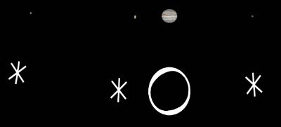
This minilesson gives 26 examples (in order of date) of Galileo’s first observations of the four major moons of Jupiter during the winter of 1610. The actual configuration of each night is beautifully displayed on the dome by Starry Night and then Galileo’s sketch is presented directly underneath it so that your audience can compare the sketch to reality. You will be astonished at Galileo’s accuracy, as well as the restrictions of his poor optics and resolution that confined his work. My students enjoy these comparisons even more than I do!
North Celestial Pole (NCP) Altitude
My students always scratch their heads when presented with the idea that the North Celestial Pole is always the same number of degrees above your horizon as your latitude. This series of overlaying diagrams attempts to clearly lay out exactly why this is the case.
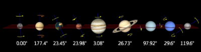
Planetary Tilts
Steve Sanders, Observatory Administrator at Eastern University and my right hand man, came up with this idea to beautifully illustrate the various planetary axis tilts side by side as well as their rotation periods. This animation is so impactful that the folks at ViewSpace used it in one of their presentations last year!
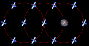
Quasars Fulldome
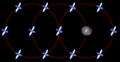
This is one of my all time favorite mind-blowing demonstrations! In a series of overlaying fulldome illustrations (again created by Steve Sanders), the second cosmological principle of the universe looking the same everywhere is demonstrated by using the appearance of quasars as seen from any galaxy, starting from the Milky Way. Your audience will be left awestruck when they discover that the Milky Way is a quasar as seen by a distant galaxy which to us looks like a quasar!
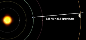
Roemer’s Method Revised
One of my favorite minilessons from Volume 1, we’ve revised this presentation with a new animation by Steve Sanders which very clearly shows the concept behind the light time effect and how Roemer was the first to demonstrate that the speed of light was finite and approximate its value. You can not only show this effect to your audience but make an incredibly precise and straightforward measurement from it of the speed of light!
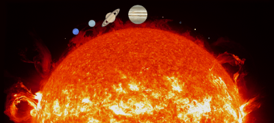
Solar System Scale Revised
I still use this minilesson in nearly every one of my presentations and for all ages. We have greatly improved the graphics used in this minilesson and I know you will like the results!
Stellar Sizes Revised
Like Solar System Scale, I use this minilesson frequently in most of my presentations, and we’ve revised it by adding a final graphic at the end which shows VY Canis Majoris in its entirety on the dome in one final scale shift.
Synodic Periods of Mercury, Venus, Mars and Jupiter
These are my favorite new additions in Volume 3! Each is a separate minilesson and carefully steps the audience through how Copernicus disentangled synodic periods of the planets into their sidereal periods around the Sun! Although very few people have ever been taught this concept, it’s very straightforward and illuminating when you see it on the dome. Test one out for yourself and you’ll be hooked!
Titius-Bode Rule
We often mention this infamous “Law” in our astronomy classes, so I wanted to present it in a historical fashion to demonstrate what effect it had on astronomer’s thinking when the Solar System was being explored and new planets being discovered. It’s the perfect example of a mathematical oddity that may or may not be scientifically meaningful. I think you will find it a fascinating subject as presented on the dome in this minilesson!
Watery Constellations
This little minilesson playfully depicts the fact that the region of the sky known as “The Sea” by the ancients has water-related constellations residing in it for a specific reason, namely that the Sun traversed this part of the sky during the rainy season in the Mediterranean. You will also be able to show your audience in a natural way that the position of the winter solstice used to be in Capricorn around 1000 BC, and hence that latitude parallel is called the Tropic of Capricorn.
Perhaps the greatest contribution to the official contents of Volume 3 is the availability of three unique fulldome interactive programs: Epicycles, Newton’s Mountain, and Tides. These three programs allow you to clearly demonstrate subjects which I have found extremely challenging for my students:
Epicycles shows many of the intricacies and systematics of the simplified Ptolemaic geocentric system and will alert your audiences to the vagaries of “saving the model at any cost.”
Newton’s Mountain is a 21st century interactive version of Newton’s attempt to explain exactly what an orbit is allowing you to show your audience in real time different orbits as a cannonball literally falls around the Earth.
Tides shows exactly why the Moon causes the water to bulge on either side of the Earth via differential gravitational forces as well as demonstrating that the bulge is not the same on both sides!
REQUIRES WINDOWS 7 ON THE RENDERBOX COMPUTER. Multi-projector systems must be based on Scaleable – not compatible with EasyBlend.
These three programs require purchase because of the many years of work which went into their development and implementation. They are now available for online purchase and immediate download:
I hope that you and your audiences thoroughly enjoy this latest addition to the Fulldome Curriculum, and that they will be helpful as you continue to strive to educate people in the subjects that we all love.
By now I hope you’re heard about the interstellar interloper that’s been passing through the inner solar system recently. This asteroid, which has been named ‘Oumuamua, is the first-ever discovered object that has been observed coming into the solar system from elsewhere in the Milky Way that is larger than tiny bits of dust.
There are several known instances of objects being “ejected” out of our solar system, so periodically there should be a chance to see a passing object that has been “ejected” from some other solar system passing by us. But only objects that pass close to the Sun or those that cast their own light are bright enough to be seen.
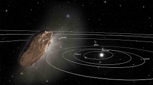
‘Oumuamua (NASA artist’s impression)
‘Oumuamua was discovered on Oct. 19th when it was already more than a month past its closest point to the Sun. It’s only about 300 feet across, and it was close enough to Earth to be seen for a short while.
Objects passing through the solar system that aren’t gravitationally bound to the Sun must be moving very quickly, although all paths are bent around their closest point to the Sun. The eccentricity of an elliptical orbit around the Sun is represented in the mathematical elements of the orbit by a number between zero and 1. The eccentricity of an object that is going too fast to be captured by the Sun has a value between 1 and infinity. The value in this case is about 1.2, and the object’s velocity entering the solar system was about 59,000 mph. It was probably ejected from another star many light years away and millions of years ago, although it is from the “disk” of the Milky Way and not the more exotic “halo”. A “halo” object would probably be moving faster.
‘Oumuamua’s orbit can be simulated in Starry Night Dome. The orbital elements are a little on the uncertain side because of the short duration of observations between discovery and it zipping out of range. And the effect of the over-unity eccentricity appears to “break” the position of the object during times before February 2016 or after March 2019. But the 3 years when it’s at its closest point to the Sun are replicated pretty well.
To add ‘Oumuamua to SciDome Version 7, right-click on the Sun in Starry Night Preflight and select ‘New Asteroid…’ and enter the following values in the details window that pops up, using the ‘Pericentric’ method instead of ‘Near-Circular.’ Also pick an appropriate name in the ‘Untitled’ field.
Once you close this details window and “keep” the new object, and quit SciDome properly, the new object will be written to a file called “User Planets.ssd”. You need to copy this file from its location on Preflight to the Renderbox for it to be “live” on both computers.
c:\Users\Spitz\AppData\Local\Simulation Curriculum\Starry Night Prefs\Preflight\User Planets.ssd
This file needs to be copied and installed on the Renderbox at the comparable folder location:
c:\Users\Spitz\AppData\Local\Simulation Curriculum\Starry Night Prefs\Renderbox\User Planets.ssd
Please contact me if you need a little extra guidance on making this work. After this is done, the object should be “live” in Starry Night on the dome during the current “Now”.
You can also fly out to the object and watch the planets and the Sun fly by as its lumpy asteroid shape zooms past. I would recommend one special piece of orientation for objects like this. During SciDome training, one of the choices we emphasize when looking at a solar system object from above is that you can “Rotate With” or “Hover Over” the planet or moon below. If you “Rotate With” while looking down at the United States, and speed up time, the Earth won’t appear to rotate, you can see successive nightfalls and daybreaks over North America, and the background stars will rotate around in the background. If you “Hover Over”, as time passes North America will rotate away to the east, Asia will appear out of the west and the fixed stars won’t move. The Sun Angle won’t change much either.
There is a third option in the dropdown menu that allows you to choose “Rotate With” or “Hover Over”, which is very much like “Hover Over” but not quite. It’s called “Follow in Orbit.” The small difference between “Hover Over” and “Follow in Orbit” is that “Follow in Orbit” will maintain the phase of illumination by the Sun as the planet orbits the Sun, and the fixed stars will slowly sweep by although the Sun Angle won’t change as time passes. “Hover Over” is completely inertial – as the planet orbits the Sun, the phase of the Sun Angle will slowly change and only the fixed stars will stay fixed.
We don’t always drill down far enough to distinguish between “Hover Over” and “Follow in Orbit” because it takes more than a month of time flow to accumulate a 30° difference between the two. But in the case of ‘Oumuamua, because its position with respect to the Sun changes so quickly, you might want a way to keep the Sun Angle constant so the source of illumination won’t rotate away from your point of view and you “lose the light”. “Follow in Orbit” is a useful orientation choice for an object like this.
A little bit of hay has been made of the way the incoming path of ‘Oumuamua leads back towards the constellation Lyra. This can also be simulated in Starry Night. The brightest star in Lyra is Vega, which was the fictional location of the first extraterrestrial signals in the Carl Sagan novel Contact. Sagan may have picked Vega to use in his book because it has been known for some time that the motion of the Sun and the solar system through the Milky Way is in the general direction of that star.
The great American/Canadian astronomer Simon Newcomb wrote in Elements of Astronomy – a book Sagan would have known – “The motion of our solar system toward the constellation Lyra is one of the most wonderful conclusions of modern astronomy.” However, as we move in the direction of that constellation, Lyra and the other stars in it have their own movements that will scramble them all out in other directions as time passes.
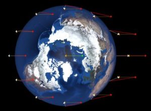
The proper motions of the stars can also be turned on in Starry Night as a series of artificial lines, and simulated back and forth through a couple of hundred thousand years of movement centered on the present if you switch to a “Stationary Location.” These proper motions may appear random, but if you highlight some of the closest and most well-known nearby stars, you can track them moving away from or toward the direction of Lyra as time passes forward or backward with some coherence.
Three long-awaited fulldome astrophysics apps created by Dr. David H. Bradstreet are now available for purchase and immediate download for installation on SciDome systems. Tides, Newton’s Mountain and Epicycles are selling for $200 individually or $500 for all three.
REQUIRES WINDOWS 7 ON THE RENDERBOX COMPUTER. Multi-projector systems must be based on Scaleable – not compatible with EasyBlend.
These programs teach the difficult concepts of tides, orbital motion, and epicycles in unique ways on your dome. All three programs are completely controllable via an intuitive interface on your Preflight computer. In addition, Tides is controllable via SciTouch for a seamless teaching experience for your audience.
The respective At A Glance teaching guides are all available for free download if you’d like to preview what you can do with these unique Fulldome interactive programs:
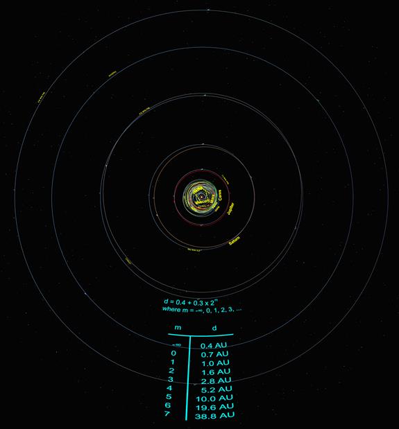
Volume 3 of the Fulldome Curriculum includes a lesson based on the Titius-Bode “Rule.” In this new teaching module we present the orbits predicted by the Titius-Bode relation in a historical timeline compared to the actual planetary orbits to show students why this apparent rule was important in 18th and 19th century astronomy.
The Titius-Bode “Rule” purports to describe an apparent mathematical correspondence in the sizes of the orbits of the classic planets in our Solar System. Although the idea of some kind of relationship had been hypothesized before Johann Daniel Titius and Johann Elert Bode, their publications in 1766 and 1772, respectively, brought this relation into the limelight of astronomical thought, and hence it is named after them.
The idea is that there is a mathematical relationship between each of the orbits of the classic planets. Usually it is presented in the following form:
d=0.4+0.3x2m
… where m = -∞, 0, 1, 2, 3,… and d is the semi major axis of the planet in astronomical units.
Historically, this relationship was believed to be revealing something intrinsic about the positioning of the planets in the Solar System, that there might have been some type of resonance phenomenon within the formation of the planets within the solar nebula. The reason for this belief came out of the astronomical discoveries which were made subsequent to its popularization in the 18th century. To see this in its historical context, let’s set up a table the way it would have been constructed in the late 1700’s:
Interesting results, but the huge gap between Mars and Jupiter posed a real problem!
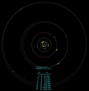
SciDome view showing Uranus’ orbit compared to the Titius-Bode prediction
Shortly after the Titius-Bode “Law” became publicized, William Herschel in 1781 discovered a new planet, Uranus! This was a paradigm changing discovery, but what was just as incredible was that its semi major axis was calculated to be 19.2 AU, nearly doubling the size of the Solar System! Just as remarkable, the next predicted semi major axis from the Titius-Bode “Law” was 19.6 AU, only 2.1% different from the measured size!
This discovery started astronomers thinking that perhaps there was more to the Titius-Bode “Law” than they once thought, that perhaps it wasn’t coincidence but was revealing a yet undiscovered physical relationship within the Solar System. Twenty years later, on the first night of the new century, 1801, Father Giuseppe Piazzi discovered a new “planet,” later named Ceres.
What was truly remarkable about this new planet was that it’s semi major axes was eventually calculated with a new mathematical method by Carl Friedrich Gauss to be 2.8 AU, nearly exactly what the Titius-Bode “Law” had predicted for a planetary body residing in the gap between Mars and Jupiter! Of course soon thereafter many more bodies were discovered to reside within the gap, and by the 1850’s these objects were renamed asteroids.
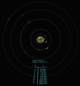
However, the belief in the Titius-Bode “Law” was gaining new proponents, since it seemed to have predicted positions in which Solar System objects were subsequently discovered! The next predicted orbit would lie at 38.8 AU, and the search was on for yet another planet! Sure enough, Neptune was discovered with the aid of Newtonian physics in 1846, but its semi major axis was 30.1 AU, notthe 38.8 AU expected from the Titius-Bode relationship.
SciDome display showing the large discrepancy between Neptune’s orbit (30.1 AU) and the predicted Titius-Bode orbit of 38.8 AU
This large discrepancy led to the virtual abandonment of the Titius-Bode relationship as a physical law. However, it’s interesting to note that when Pluto was discovered in 1930 its semi major axis was determined to be 39.5 AU, very close to the previously expected distance. Of course Pluto has now been relegated to dwarf planet status because of the myriad of new objects which have been discovered in the Kuiper Belt.
The next expected semi major axis from the Titius-Bode relationship is 77.2 AU. And isn’t it interesting that Sedna’s perihelion distance is 76.1 AU, although its semi major axis is a whopping 506.8 AU!
The moral of the story seems to be that although the Titius-Bode relationship has never been convincingly proven to come from physical laws, it is noteworthy historically but also serves to perhaps warn us about jumping to conclusions even though the initial evidence may seem inviting. The Titius-Bode relationship is today such a controversial topic that Icarus, the main professional journal for presenting papers on Solar System dynamics, refuses to publish any articles on the subject!
Our ancestors were highly intelligent people who devised ingenious methods to model what they perceived to be reality in the skies. Unfortunately, they came at many of these observations with deep-rooted prejudices and a priori (preconceived) beliefs which shackled their creativity.
Figure 1: Close up of the Ptolemaic system out to the Sun’s sphere
The prevalent, far-reaching belief was that the Earth was immovable and at the center of the universe. Of course we know this is preposterous (even to the point that there is no such thing as a center to the universe), it is still a useful exercise to challenge students to prove, without leaving the Earth or using satellites, that the Earth does indeed rotate and that it revolves about the Sun.
Another a priori assumption was that celestial bodies never stopped moving, as opposed to “earthly” objects which eventually came to a halt. So, when the planets periodically went back and forth in the sky, this was unacceptable and Apollonius of Perga came up with a “solution” that allowed the wanderers to be always moving without stopping by coupling two motions at once. The planets were not simply attached to a mystical sphere (“deferent”) but they were actually attached to a mini-sphere (“epicycle”) which rotated on the larger one.
Figure 2: Mercury’s retrograde path in the Ptolemaic system
In this way planets could move around the sky but intersperse that generally easterly motion with apparent backwards motion (retrograde) when the transparent epicycle carried the planet backwards. The ancients latched on to it and it was greatly preferred to having deferents slow down, stop, go backwards, stop, then resume their original direction.
My colleague David Steelman and I created a program called Epicycles for SciDome that illustrates the main characteristics of the Ptolemaic Geocentric Model. It helps students discover the systemics of the model which can only be explained as “it just has to be that way”. Whenever that is the reasoning, it signals a problem with the theory/model. This will become obvious as we go through this paper.
Let’s first take a close look at the bodies closest to the Earth in the geocentric model, as shown in Figure 1.
The Moon moves the fastest in the sky (and even changes shape!) so it was assumed to be closest to Earth. Placement of Mercury and Venus closer to the Earth than the Sun was problematic. The theory was based upon the idea that those that appeared to move the slowest must be farthest away from Earth. The problem is that the epicycle containing Mercury, the epicycle containing Venus, and the Sun all orbited around the Earth in one year! So their order was reluctantly agreed upon because Mercury moved fastest on it epicycle, Venus next fastest, and of course the Sun had no epicycle (because it never retrograded).
Figure 3: Venus and Mercury’s retrograde paths in the Ptolemaic system
The epicycle sizes are based on arbitrarily assumed distances from Earth. The angles had to match the size of the retrograde loops seen in the sky so, looking at Figure 1, Mercury’s epicycle is tiny compared to Venus’ because Mercury’s retrograde loop is about 52 degrees in extent whereas Venus’ is about 92 degrees! The fact that Venus is farther away than Mercury from the Earth in this model requires it to be considerably larger than one might expect, but these are to scale to create the properly sized retrograde patterns.
As time is progressed a trace can be turned on which shows the retrograding patterns of the planets. Figure 2 shows a close up of Mercury and Figure 3 that of Venus.
When I ask students if they see anything peculiar as time progresses, eventually someone notices that the centers of the epicycles of Mercury and Venus are exactly and always lined up with the line connecting the Earth and Sun (the Earth-Sun Line). What explanation would the ancients have given for this? “It just has to be this way for this model to work.” Red flag number 1 that there’s something wrong with this theory.
Figure 4: The planets beyond the Sun’s sphere
Of course we know that in the Copernican heliocentric model we don’t need epicycles to cause Mercury and Venus to wobble back and forth around the Sun because they are simply closer to the Sun than Earth and they orbit the Sun. In fact, Copernicus was the first to completely untangle the motions of Mercury and Venus from the Sun’s motion.
This confusion is one rarely-discussed reason why the Copernican heliocentric model was so appealing. It unambiguously separated the motions of Mercury and Venus and even established, for the first time, their orbital periods around the Sun (88 days and 225 days, respectively).
Now observe the planets beyond the Sun, as shown in Figure 4. As we advance time another strange systematic displays itself, although this one is a lot more challenging to pick out. The Earth-Sun Line is always parallel to the planet’s epicycle radius! You can easily see this in Figure 4 now that you know to look for it.
Again, the ancients noted this “coincidence” but could never explain it other than “it has to be this way for the model to work.” Another red flag has raised itself in the flawed Ptolemaic model! The basic reason for this “coincidence” is because the retrograde motion of each planet is a function of its position relative to the Earth in its own orbit. Since we’re locking down the Earth and moving the Sun, it’s the orientation of the Earth-Sun Line that is the determining factor as to when planets exhibit their retrograde motions.
Figure 5 – The retrograde paths of the planets beyond the Sun’s sphere
When the planets leave breadcrumbs (see Figure 5) their retrograding paths become obvious. Again, the model has been carefully defined to accurately recreate the width of the retrograde loops as well as their frequency.
This is a fun and thought provoking lesson for my students because it demonstrates how intelligent and clever the ancients were in mimicking celestial motions, but it also shows how preconceived notions can weigh one down and severely complicate the model. It also clearly points out that when certain “features” of a model have no other explanation than “it has to be that way for the model to work” that the model is most likely flawed or incorrect at its core. But having the Earth move was a huge paradigm shift, and it took over 1500 years to overthrow it!
 This minilesson gives 26 examples (in order of date) of Galileo’s first observations of the four major moons of Jupiter during the winter of 1610. The actual configuration of each night is beautifully displayed on the dome by Starry Night and then Galileo’s sketch is presented directly underneath it so that your audience can compare the sketch to reality. You will be astonished at Galileo’s accuracy, as well as the restrictions of his poor optics and resolution that confined his work. My students enjoy these comparisons even more than I do!
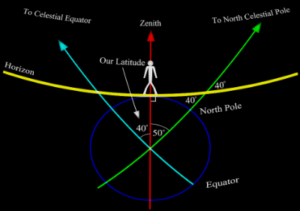
 I still use this minilesson in nearly every one of my presentations and for all ages. We have greatly improved the graphics used in this minilesson and I know you will like the results!
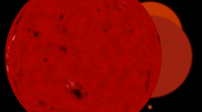 Like Solar System Scale, I use this minilesson frequently in most of my presentations, and we’ve revised it by adding a final graphic at the end which shows VY Canis Majoris in its entirety on the dome in one final scale shift.
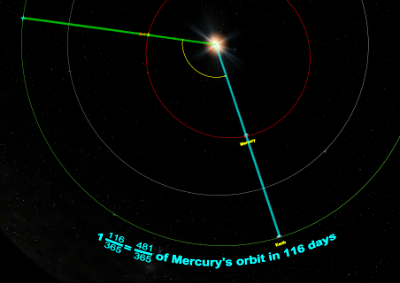 These are my favorite new additions in Volume 3! Each is a separate minilesson and carefully steps the audience through how Copernicus disentangled synodic periods of the planets into their sidereal periods around the Sun! Although very few people have ever been taught this concept, it’s very straightforward and illuminating when you see it on the dome. Test one out for yourself and you’ll be hooked!
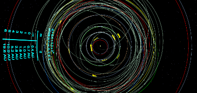 We often mention this infamous “Law” in our astronomy classes, so I wanted to present it in a historical fashion to demonstrate what effect it had on astronomer’s thinking when the Solar System was being explored and new planets being discovered. It’s the perfect example of a mathematical oddity that may or may not be scientifically meaningful. I think you will find it a fascinating subject as presented on the dome in this minilesson!
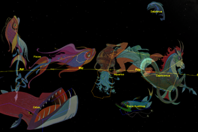

 Three long-awaited fulldome astrophysics apps created by Dr. David H. Bradstreet