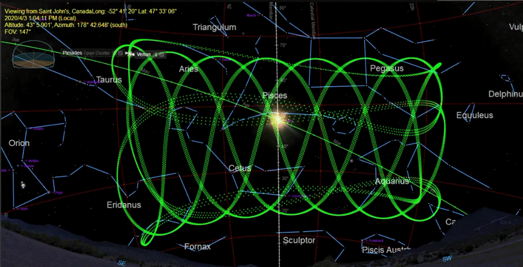
There is an upcoming event in the evening sky that is worth notifying your colleagues about on social media this week. Venus is going to pass in front of the Pleiades star cluster on Friday, April 3rd. The neat thing about it is that this happens every 8 years, to the day. You can simulate it on SciDome in Starry Night.
Venus is the brightest object in the evening sky other than the Moon this month, and it is provoking lots of UFO reports. Venus is also getting closer to Earth, so its apparent size is growing. Venus is also starting to turn into a crescent as it gets between the Earth and the Sun. It is a fascinating object to observe through small binoculars, especially when the Pleiades are also visible in the same binocular field of view.
Venus orbits the Sun every 225 days, but the Earth orbits the Sun as well, and it takes more than a year for Venus to catch up to the Earth and pass us. Venus returns to the same position with respect to the Earth every 8/5ths (or 1.6) of a year, or 584 days. Because it’s not equal to a year, when Venus returns after 584 days, it’s not in position against the same background stars. However, the lowest integer multiple of 1.6 is 8, so Venus does appear against the same background stars on the date when it passes the Earth every 8 years (although a backwards drift of 2 days per 8 years accumulates.)
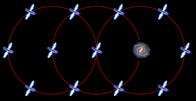
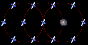
We’re familiar with the analemma, the figure-8 pattern the Sun draws on the sky if you animate Starry Night forward in steps of 1 day at noon. Venus also has an analemma, but it’s a spirograph pattern instead of a figure-8 because its Synodic period repeats five times over the course of those 8 years. This spirograph pattern of Venus’s Local Path at 1-day intervals in Starry Night is really cool.
The Synodic Period of Venus is covered in depth in David Bradstreet’s Fulldome Curriculum Vol. 3 minilesson “Synodic Period of Venus”.
The Pleiades is the brightest star cluster that happens to be on the Ecliptic plane, so it can periodically be occulted by the Moon, and the planets sometimes pass through it. Venus passes by the Pleiades every 8/5ths of a year too, although sometimes it passes by when the Pleiades is near the Sun in May, and sometimes when the Pleiades is in the predawn sky in late summer, and sometimes it passes by the Pleiades twice because it has a retrograde loop. The accumulating 2-day error also means that Venus’s path through the Pleiades is never quite the same with each 8-year interval, and the event is a coincidence that doesn’t look so perfect if you dial it back way into the past, or well into the future. But different dates become prominent for Venus meeting the Pleiades instead.
Venus’s greatest meeting in the sky is the Transit of Venus across the face of the Sun, which is very rare, and the Transit of Venus is also affected by that accumulating drift. Venus was in front of the Sun on June 8th, 2004 and again on June 6th, 2012, but another Transit will not happen again on June 4th, 2020 (but it will be close!) The next Transit of Venus will be on December 10th, 2117.
The first time I observed Venus in the Pleiades was on April 3rd, 1996, and I recommend you look up that date in Starry Night especially. Also on that date in the evening there was a total lunar eclipse in the eastern sky, and also the bright Comet Hyakutake was in the western sky just a few degrees away from the Pleiades.
So please make your community aware of the coincidence of Venus and the Pleiades this week, so they can look up again on April 3rd of 2028 and remember what they were doing 8 years earlier.
Earlier this month, another “multi-messenger” announcement was made of the discovery of a new astronomical outburst by different instruments that study different parts of the universe. The first major multi-messenger astronomy discovery was announced last year after the collision of two neutron stars was observed in the nearby galaxy NGC 4993. The neutron star collision was observed first with the LIGO and Virgo gravitational wave detectors, coincident with a gamma ray burst detected by the Fermi space telescope, pinpointed with an optical telescope in South America, and followed up with different kinds of detectors.
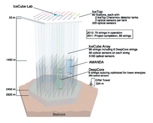
This new announcement is based on the detection of a very unusual neutrino or “ghost particle” at the IceCube Neutrino Observatory at the South Pole. This event is worth pointing out in SciDome because we have a horizon panorama that matches the horizon at the South Pole, and one or two other points that may help students understand how the sky works and what neutrinos are.
Neutrinos have been observed with detectors in both the northern and southern hemispheres of Earth, and they are created as a byproduct of various nuclear reactions. Neutrinos hardly interact with normal matter at all, and they tend to radiate outwards from their point of creation at the speed of light.
Neutrinos at rest were assumed to be massless until evidence to the otherwise shown by Art McDonald and Raymond Davis, Jr., led to them being awarded the Nobel Prize in Physics in 2015.
The interaction of neutrinos with normal matter is so weak that most neutrinos that encounter the Earth fly straight through it without hitting anything. In February 1987 when a nearby supernova popped off in the Large Magellanic Cloud, 25 neutrinos were detected at neutrino observatories in the northern hemisphere, where the Large Magellanic Cloud never rises above the horizon.
The new neutrino detection from IceCube at the South Pole was detailed enough to provide a vector back to its point of origin, somewhere within a 1.3-degree-wide circle on the sky.
The Spitz Fulldome Curriculum, included with every SciDome system, includes dozens of lessons prepared by noted astronomy educator Dr. David Bradstreet
The circle enclosed a radio source discovered in 1983, a galaxy 3.7 billion light years away with an active supermassive black hole at its core. This is one of the quasars like Dr. Bradstreet uses in his “Quasars Fulldome” show from the Fulldome Curriculum Vol. 3. Because this quasar’s jet is pointed at us, it is called a “blazar”; this term originated because the first of its type happened to be named “BL Lacertae”, and because blazars can appear brighter than normal quasars and their brightness can vary more quickly than normal quasars.
Like before, this neutrino detected from the South Pole had flown through the Earth to get to the detector. The blazar TXS 0506+056 is located at about 5 hours right ascension and +5° north of the celestial equator. Only objects south of the celestial equator are above the horizon as seen from the South Pole.
TXS 0506+056 is conveniently located in the Shield of Orion, part of the most easily recognized equatorial constellation on the sky. The blazar is labeled “MG 0509 +0541” in SciDome and is one of the quasars in Dr. Bradstreet’s “Galactocentric Distributions” minilesson.
In the part of the Fulldome Curriculum “Seasons” class that visits the South Pole, the audience may have a hard time recognizing Orion because it is upside down and its northern half, including TXS 0506+056 is below the horizon. The horizon needs to be switched off and then tilted up to bring the rest of the constellation into view to simulate a “neutrino filter”.
The prefix TXS stands for ‘Texas’, where UT-Austin astronomers set up a radio telescope array outside of Marfa for several years in the 1980s – now removed. MG stands for ‘MIT-Green Bank Observatory’.
The mass of neutrinos and other particles is calculated in electron volts, but because they are so small, only particles that have a large amount of kinetic energy are comparable to things that we can comprehend. 1 trillion electron volts (1 TeV using the prefix tera-) is comparable to the kinetic energy of a mosquito in flight. The most powerful cosmic ray ever detected had a mass of 300 quintillion electron volts, comparable to a pitched baseball.
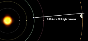
The single neutrino detected by IceCube from TXS 0506+056 had a mass of 290 TeV. After crossing 3.7 billion light years in space, this is by far the most distant neutrino emission ever detected: the only other objects in the sky that have produced detected neutrinos have been the Sun (8 light-minutes away) and Supernova 1987A (168,000 light-years.)
(In 2012, the IceCube Collaboration detected three other high-energy neutrinos, which they named Bert, Ernie and Big Bird, but where Bert and Ernie came from is not known, and Big Bird was probably generated by the blazar PKS B1424-418 with a certainty of 95%. That’s only two sigma, which does not hold water with particle physicists who have much stricter statistical significance limits. TXS 0506+56 was much more narrowly confined.)
Because matter and energy are relative, an electron volt is equivalent to the energy exchanged by the charge of a single electron moving across an electric potential difference of one volt. The only way a neutrino can be detected is on the rare occasion when it enters a neutrino detector (like a large underground tank of heavy water or tetrachloroethylene or linear alkylbenzene or another chemical) and collides with an atomic nucleus or an electron inside the detector, emitting light that can be detected with photomultiplier tubes. IceCube is unusual because its detectors have been drilled into the Antarctic ice pack and are not suspended in water or another fluid.
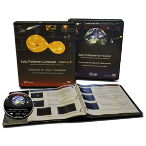
I’m excited to announce that Volume 3 of the Spitz Fulldome Curriculum is being released to all SciDome users, and will of course be automatically incorporated into all future SciDome installations. We thought that this would be an opportune time to give a very brief overview of what’s contained in this volume. There are several revisions to previous minilessons as well as several all new offerings:
Galilean Moons
This minilesson gives 26 examples (in order of date) of Galileo’s first observations of the four major moons of Jupiter during the winter of 1610. The actual configuration of each night is beautifully displayed on the dome by Starry Night and then Galileo’s sketch is presented directly underneath it so that your audience can compare the sketch to reality. You will be astonished at Galileo’s accuracy, as well as the restrictions of his poor optics and resolution that confined his work. My students enjoy these comparisons even more than I do!
North Celestial Pole (NCP) Altitude
My students always scratch their heads when presented with the idea that the North Celestial Pole is always the same number of degrees above your horizon as your latitude. This series of overlaying diagrams attempts to clearly lay out exactly why this is the case.
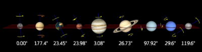
Planetary Tilts
Steve Sanders, Observatory Administrator at Eastern University and my right hand man, came up with this idea to beautifully illustrate the various planetary axis tilts side by side as well as their rotation periods. This animation is so impactful that the folks at ViewSpace used it in one of their presentations last year!
Quasars Fulldome
This is one of my all time favorite mind-blowing demonstrations! In a series of overlaying fulldome illustrations (again created by Steve Sanders), the second cosmological principle of the universe looking the same everywhere is demonstrated by using the appearance of quasars as seen from any galaxy, starting from the Milky Way. Your audience will be left awestruck when they discover that the Milky Way is a quasar as seen by a distant galaxy which to us looks like a quasar!
Roemer’s Method Revised
One of my favorite minilessons from Volume 1, we’ve revised this presentation with a new animation by Steve Sanders which very clearly shows the concept behind the light time effect and how Roemer was the first to demonstrate that the speed of light was finite and approximate its value. You can not only show this effect to your audience but make an incredibly precise and straightforward measurement from it of the speed of light!
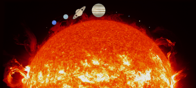
Solar System Scale Revised
I still use this minilesson in nearly every one of my presentations and for all ages. We have greatly improved the graphics used in this minilesson and I know you will like the results!
Stellar Sizes Revised
Like Solar System Scale, I use this minilesson frequently in most of my presentations, and we’ve revised it by adding a final graphic at the end which shows VY Canis Majoris in its entirety on the dome in one final scale shift.
Synodic Periods of Mercury, Venus, Mars and Jupiter
These are my favorite new additions in Volume 3! Each is a separate minilesson and carefully steps the audience through how Copernicus disentangled synodic periods of the planets into their sidereal periods around the Sun! Although very few people have ever been taught this concept, it’s very straightforward and illuminating when you see it on the dome. Test one out for yourself and you’ll be hooked!
Titius-Bode Rule
We often mention this infamous “Law” in our astronomy classes, so I wanted to present it in a historical fashion to demonstrate what effect it had on astronomer’s thinking when the Solar System was being explored and new planets being discovered. It’s the perfect example of a mathematical oddity that may or may not be scientifically meaningful. I think you will find it a fascinating subject as presented on the dome in this minilesson!
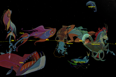
Watery Constellations
This little minilesson playfully depicts the fact that the region of the sky known as “The Sea” by the ancients has water-related constellations residing in it for a specific reason, namely that the Sun traversed this part of the sky during the rainy season in the Mediterranean. You will also be able to show your audience in a natural way that the position of the winter solstice used to be in Capricorn around 1000 BC, and hence that latitude parallel is called the Tropic of Capricorn.
Perhaps the greatest contribution to the official contents of Volume 3 is the availability of three unique fulldome interactive programs: Epicycles, Newton’s Mountain, and Tides. These three programs allow you to clearly demonstrate subjects which I have found extremely challenging for my students:
Epicycles shows many of the intricacies and systematics of the simplified Ptolemaic geocentric system and will alert your audiences to the vagaries of “saving the model at any cost.”
Newton’s Mountain is a 21st century interactive version of Newton’s attempt to explain exactly what an orbit is allowing you to show your audience in real time different orbits as a cannonball literally falls around the Earth.
Tides shows exactly why the Moon causes the water to bulge on either side of the Earth via differential gravitational forces as well as demonstrating that the bulge is not the same on both sides!
REQUIRES WINDOWS 7 ON THE RENDERBOX COMPUTER. Multi-projector systems must be based on Scaleable – not compatible with EasyBlend.
These three programs require purchase because of the many years of work which went into their development and implementation. They are now available for online purchase and immediate download:
I hope that you and your audiences thoroughly enjoy this latest addition to the Fulldome Curriculum, and that they will be helpful as you continue to strive to educate people in the subjects that we all love.
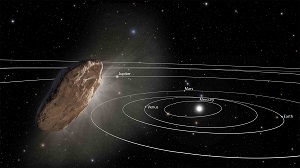
By now I hope you’re heard about the interstellar interloper that’s been passing through the inner solar system recently. This asteroid, which has been named ‘Oumuamua, is the first-ever discovered object that has been observed coming into the solar system from elsewhere in the Milky Way that is larger than tiny bits of dust.
There are several known instances of objects being “ejected” out of our solar system, so periodically there should be a chance to see a passing object that has been “ejected” from some other solar system passing by us. But only objects that pass close to the Sun or those that cast their own light are bright enough to be seen.
‘Oumuamua (NASA artist’s impression)
‘Oumuamua was discovered on Oct. 19th when it was already more than a month past its closest point to the Sun. It’s only about 300 feet across, and it was close enough to Earth to be seen for a short while.
Objects passing through the solar system that aren’t gravitationally bound to the Sun must be moving very quickly, although all paths are bent around their closest point to the Sun. The eccentricity of an elliptical orbit around the Sun is represented in the mathematical elements of the orbit by a number between zero and 1. The eccentricity of an object that is going too fast to be captured by the Sun has a value between 1 and infinity. The value in this case is about 1.2, and the object’s velocity entering the solar system was about 59,000 mph. It was probably ejected from another star many light years away and millions of years ago, although it is from the “disk” of the Milky Way and not the more exotic “halo”. A “halo” object would probably be moving faster.
‘Oumuamua’s orbit can be simulated in Starry Night Dome. The orbital elements are a little on the uncertain side because of the short duration of observations between discovery and it zipping out of range. And the effect of the over-unity eccentricity appears to “break” the position of the object during times before February 2016 or after March 2019. But the 3 years when it’s at its closest point to the Sun are replicated pretty well.
To add ‘Oumuamua to SciDome Version 7, right-click on the Sun in Starry Night Preflight and select ‘New Asteroid…’ and enter the following values in the details window that pops up, using the ‘Pericentric’ method instead of ‘Near-Circular.’ Also pick an appropriate name in the ‘Untitled’ field.
Once you close this details window and “keep” the new object, and quit SciDome properly, the new object will be written to a file called “User Planets.ssd”. You need to copy this file from its location on Preflight to the Renderbox for it to be “live” on both computers.
c:\Users\Spitz\AppData\Local\Simulation Curriculum\Starry Night Prefs\Preflight\User Planets.ssd
This file needs to be copied and installed on the Renderbox at the comparable folder location:
c:\Users\Spitz\AppData\Local\Simulation Curriculum\Starry Night Prefs\Renderbox\User Planets.ssd
Please contact me if you need a little extra guidance on making this work. After this is done, the object should be “live” in Starry Night on the dome during the current “Now”.
You can also fly out to the object and watch the planets and the Sun fly by as its lumpy asteroid shape zooms past. I would recommend one special piece of orientation for objects like this. During SciDome training, one of the choices we emphasize when looking at a solar system object from above is that you can “Rotate With” or “Hover Over” the planet or moon below. If you “Rotate With” while looking down at the United States, and speed up time, the Earth won’t appear to rotate, you can see successive nightfalls and daybreaks over North America, and the background stars will rotate around in the background. If you “Hover Over”, as time passes North America will rotate away to the east, Asia will appear out of the west and the fixed stars won’t move. The Sun Angle won’t change much either.
There is a third option in the dropdown menu that allows you to choose “Rotate With” or “Hover Over”, which is very much like “Hover Over” but not quite. It’s called “Follow in Orbit.” The small difference between “Hover Over” and “Follow in Orbit” is that “Follow in Orbit” will maintain the phase of illumination by the Sun as the planet orbits the Sun, and the fixed stars will slowly sweep by although the Sun Angle won’t change as time passes. “Hover Over” is completely inertial – as the planet orbits the Sun, the phase of the Sun Angle will slowly change and only the fixed stars will stay fixed.
We don’t always drill down far enough to distinguish between “Hover Over” and “Follow in Orbit” because it takes more than a month of time flow to accumulate a 30° difference between the two. But in the case of ‘Oumuamua, because its position with respect to the Sun changes so quickly, you might want a way to keep the Sun Angle constant so the source of illumination won’t rotate away from your point of view and you “lose the light”. “Follow in Orbit” is a useful orientation choice for an object like this.
A little bit of hay has been made of the way the incoming path of ‘Oumuamua leads back towards the constellation Lyra. This can also be simulated in Starry Night. The brightest star in Lyra is Vega, which was the fictional location of the first extraterrestrial signals in the Carl Sagan novel Contact. Sagan may have picked Vega to use in his book because it has been known for some time that the motion of the Sun and the solar system through the Milky Way is in the general direction of that star.
The great American/Canadian astronomer Simon Newcomb wrote in Elements of Astronomy – a book Sagan would have known – “The motion of our solar system toward the constellation Lyra is one of the most wonderful conclusions of modern astronomy.” However, as we move in the direction of that constellation, Lyra and the other stars in it have their own movements that will scramble them all out in other directions as time passes.
The proper motions of the stars can also be turned on in Starry Night as a series of artificial lines, and simulated back and forth through a couple of hundred thousand years of movement centered on the present if you switch to a “Stationary Location.” These proper motions may appear random, but if you highlight some of the closest and most well-known nearby stars, you can track them moving away from or toward the direction of Lyra as time passes forward or backward with some coherence.
On August 17th, the Laser Interferometer Gravitational-Wave Observatory, or “LIGO”, detected gravity waves produced by the merger of two neutron stars. There are lots of good takes on this story, and it’s important that we keep retelling it in interesting ways. This entry briefly summarizes the observations of the event, while focusing in on a couple of ways that a SciDome planetarium show about this could be exciting for an educational audience.
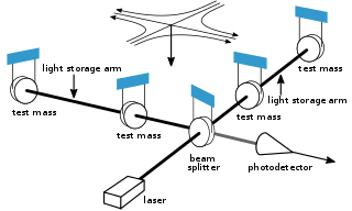
Basic components of a gravitational wave detector
A neutron star is the typical remnant left behind after a supernova explosion. Specifically, this is the kind of supernova that overtakes a massive star at the end of its lifespan, when heavy elements have accumulated at its core. Massive stars that go supernova tend to have short lifespans on the cosmic scale, only a few million years.
In a supernova, the outer layers of the star collapse onto the core, compress it, and rebound outwards in an explosion. The core is left behind, but the pressure of the infalling layers squeeze it to the point that normal matter made up of atoms can no longer exist. It is squeezed so tight that orbiting electrons and core protons violate the Pauli Exclusion Principle and combine into neutrons that have no net charge.
A neutron star is a small but extremely massive object made up of this “neutron-degenerate matter” that has no protons or electrons, with no space in between the nuclei. “Neutronium” is extremely dense, so that a teaspoon full of it would weigh two billion tonnes. The diameter of the neutron star is only a few miles.
The type of supernova that can create a neutron star tends to occur in a given galaxy roughly once per century. Neutron stars that rotate can be observed in radio waves as “pulsars”. Due to the law conservation of angular momentum on a rapidly collapsing massive object, pulsars tend to rotate extremely quickly.
The Spitz Fulldome Curriculum, included with every SciDome system, includes dozens of lessons prepared by noted astronomy educator Dr. David Bradstreet
You can review the lesson plan for the Fulldome Curriculum minilesson in your SciDome named “Galactocentric Distributions”, which has a step that highlights the locations of supernova remnants like pulsars. That ATM-4 lesson uses the Starry Night database “Supernova Remnants” which can also be toggled on and off manually.
Although neutron stars are rare (one such may be created in a galaxy of 100 billion stars after an interval of 100 years), it is possible for two pulsars to be observed orbiting each other. Since they were first observed in 1967, hundreds of pulsars have been observed in the Milky Way, and there is also a suspected population of neutron stars that can’t be observed. So far there are two known binary pulsars in the Milky Way.
Until LIGO was completed in 2002 and then upgraded in 2015, the only method of observing the effects of gravitational waves was to use a radio telescope to time the regular pulses of a binary pulsar and measure its rate of slowing. Einstein’s general theory of relativity describes gravity as a warping of space/time around massive objects. As a pair of pulsars orbit each other, some of their rotational energy is carried away by the propagation of gravitational waves. The first known binary pulsar has an orbital period of about 7 hours, and the timing of its pulses has revealed a small orbital contraction. That pair may take 300 million years to spin together.
Since LIGO was upgraded in 2015, it has started to discover gravitational wave events caused by black holes merging. Mergers of stellar-mass black holes are somewhat common in the deep cores of galaxies and maybe some other places in the universe, but so far no black hole mergers have been observed by LIGO with enough accuracy to find their host galaxies.
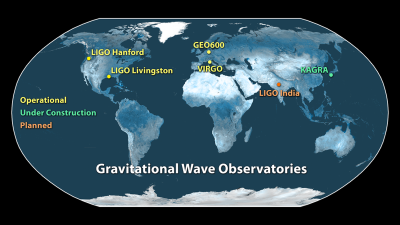
The two stations of LIGO are located in eastern Washington state and in rural Louisiana. The sensitivity of the system has recently been improved through collaboration with the European gravitational wave observatory Virgo, located outside Pisa, Italy. These locations can be visited in SciDome with The Layered Earth.
The August 17th event that’s now in the news (GW170817) was the collision of a pair of neutron stars in another galaxy. It is notable because it’s the first observed neutron star collision, and because its optical component was found thanks to triangulation between gravitational wave observatories and gamma-ray observatories.
One aspect of the breaking nature of the story is that although the news was embargoed from distribution until this week, rumors have been circulating about it since the day it happened, a few days before the total solar eclipse in August. Now that the papers have been published, notably B.P. Abbott et al. in Physical Review Letters, the scale of the collaboration becomes apparent. There are so many co-authors on these papers that it has been guesstimated that 15% of all professional astronomers are being cited. No wonder it was difficult for them to keep a secret!
The rapid outburst and the quick dimming of the object was less impressive than a supernova – maybe only a tenth as bright as a supernova, so the name “kilonova” has been proposed to distinguish this kind of an event from a supernova.
https://www.youtube.com/watch?v=nziW8fywwmg
ESO animation: Zooming in on the NGC 4993 kilonova
The host galaxy is also very close to us. One of my other hats apart from Spitz is as a supernova hunter. I’ve co-discovered ten supernovae by searching through images of external galaxies, and although it is not atypical for one or even two supernovae per year to turn up in galaxies that are less than ten million light years away, I have never found one that was closer than 215 million light years. The host galaxy, NGC 4993, is only about 120 million light years away.
NGC 4993 is so close that it was observed visually in the late 18th Century, before photography was invented, with an 18-inch reflecting telescope with a speculum metal mirror. The greatest father-and-son team of astronomers in history – William and John Herschel – found it 45 years apart.
Did I mention that neutron star collisions are rare? A given galaxy may only host a binary neutron star collision once per 100,000 years, and there are only on the order of 100,000 galaxies in the volume with radius 120 million light years.
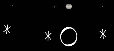
You can look up NGC 4993 in Starry Night and dial up the location and the date of its discovery: Slough, England on March 26th, 1789. This galaxy isn’t easy to see from so far north. It only gets 16° above the southern horizon as seen from Slough.
You can also dial up the discovery date of the gravitational wave event – August 17th of this year. One of the points that’s been made is that in August, NGC 4993 sets a couple of hours after the Sun, and is not easy to find in the short time available after sunset. By the time of this week’s announcement, NGC 4993 has gone behind the Sun and no new observations can be made by anybody until it returns in the predawn sky. If the gravitational waves event had happened two months later, the source of GW170817 would not have been found.
You can also fly out to the host galaxy to observe it in three dimensions with Starry Night. The name NGC 4993 is not “flyable”, so we have to type in the name that is attached to this galaxy in one of the newer catalogs that renders it as a 3D object. In the search field, type in:
The phrase “We are star stuff” has been a part of the astronomer’s public outreach lexicon for many years, since Carl Sagan. We know how to point out that all the heavy elements that make up solid matter on Earth were fused out of lighter elements in the cores of stars, and that iron and everything heavier than it was produced by supernova explosions. It’s now time to re-invent the part of this expression that deals with a lot of those heavy elements.
The neutron star collision in NGC 4993 seems to have produced more than 10 Earth masses of gold, platinum and other precious metals. Dr. Jennifer Johnson from The Ohio State University, a SciDome user, posted a Periodic Table of the Elements on her blog that has been broken down to highlight which elements can be generated by supernovae, colliding neutron stars, etc.
Novae and supernovae are among the most energetic phenomena encountered in the galaxy. Planetarium educators can simulate a number of historical nova and supernova events on SciDome using Starry Night Dome Version 7.
The following 10 transient objects can be investigated in Starry Night 7’s “Historical Supernovae” database on’s :
SN 1987A (Progenitor: Sanduleak -69° 202)
Supernova 1680 (Cassiopeia A)
SN 1604 (Kepler’s Star)
SN 1572 (Tycho’s Star)
SN 1181
SN 1054 (Crab Nebula)
SN 1006
SN 393 (G347.3-0.5)
SN 386 (G11.2-0.3)
SN 185 (RCW 86)
Each of these supernova simulations behave in one of two ways on the dome.
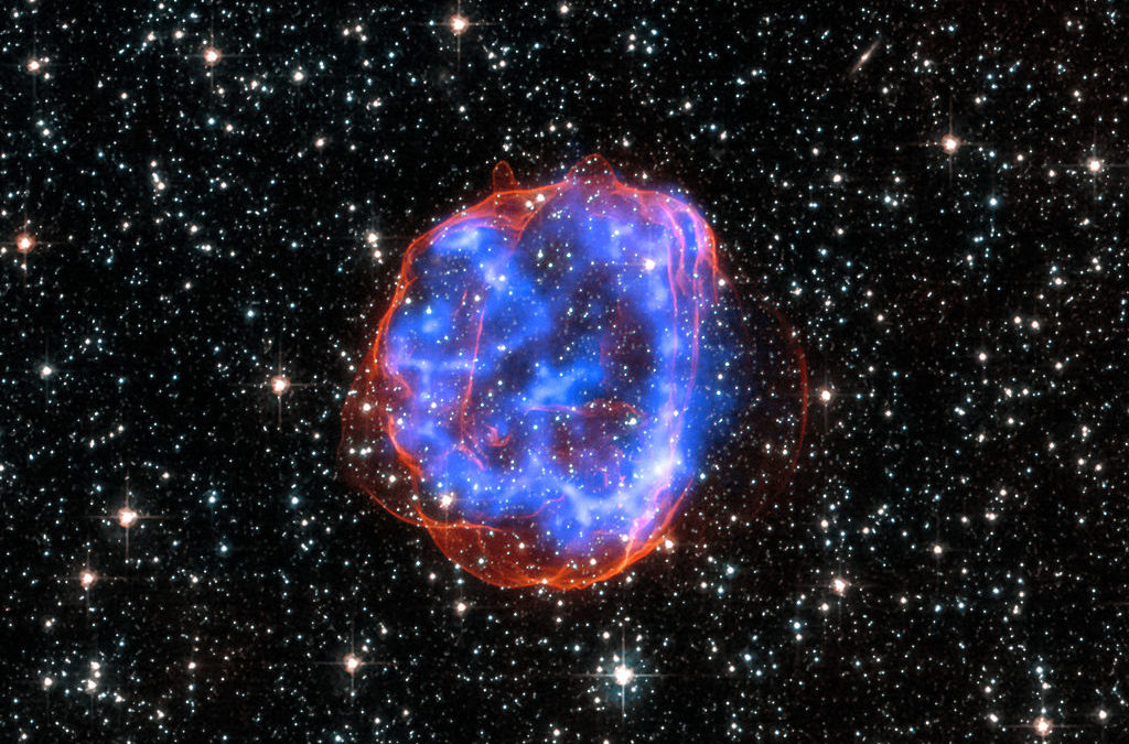
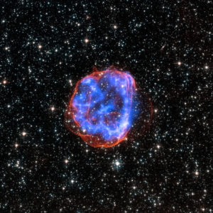
The supernovae of the years 1987, 1604, 1572, 1181, 1054 and 1006 in the Common Era were all relatively well-studied when they were visible, and their positions have been correlated with current supernova remnants. These objects are best treated in SciDome: if you look at the sky on the date they appeared and in the correct position, toggling backward and forward several days, the “Guest Star” phenomenon makes the supernova pop into existence, flare up slightly, and then fade away over the course of several months.
The supernovae of the years 1680, 393, 386 and 185 were not well-observed at the time we estimate they exploded due to interstellar dust blocking their light, the difficulty of keeping reliable extremely old observing records, etc. However, some unconfirmed observing reports claim they were observed, and their positions correlate well with supernova remnants or pulsars detected with X-ray telescopes. With no firm dates or estimated brightnesses, it’s appropriate that their positions should be marked, but these four objects do not flare up and then dim out like the first six. There are also photos of the supernova remnants docked in position over these transients in Starry Night.
How about adding objects to this database manually? That’s not so hard, and there are several candidates that have similarities to historical supernovae (although the above ten are the only recorded historical supernovae that have been as bright as the brightest stars).
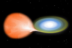
Artist’s conception of a white dwarf accreting hydrogen from a larger companion
If a supernova is a star that explodes completely, a nova is a star that is only partly exploding. There are a few different theories to describe the processes in a nova star. The most common is that a white dwarf star and a normal star are orbiting each other, and the normal star is close enough to deposit some outflowing gas on to the surface of the white dwarf. The gas builds up on the surface of the white dwarf star until it becomes unstable and explodes. The white dwarf star survives the explosion. These novae can even re-occur once the gas builds up again.
Today is the 99th anniversary of the appearance of the “Victory Star”, also known as Nova Aquilae 1918 or V603 Aquilae. For several days this star was the brightest nova in the age of the telescope, magnitude -0.5, as bright as the brightest stars. It faded back to obscurity quickly. It was known as the Victory Star because some saw it as a portent of the end of the Great War. Also, in an extreme coincidence, it appeared on the same day in June 1918 as a total eclipse of the Sun was seen from coast to coast across the United States.
The file that encodes the Historical Supernovae database is in the Sky Data folder for Starry Night 7 on both Preflight and Renderbox. This feature is not available in Starry Night 6. To make a change, both files need to be edited in an identical fashion.
Here is the code that can simulate the Nova 1918 star by pasting into a new “11th” paragraph:
The Right Ascension and Declination (RA and Dec) co-ordinates of the new star have to be entered in decimal hours and decimal degrees. The values in the line with the tag “00011_RA_Dec_DistanceLY” are accurate to put the nova in western Aquila several degrees above the asterism of stars that makes up the “foot” of the Eagle.
Some of the above values are just copied from an earlier part of the file, but the observing period, expressed in Julian dates, is shorter than for a supernova. There are only 248 days between the date 2421752 (representing June 8, 1918) and 2422000 when we can estimate the new star had dimmed below the threshold of visibility.
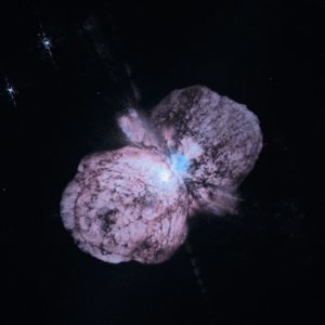
The Homunculus Nebula, surrounding Eta Carinae
There are several other nova stars that can be shoe-horned into this database. For example, the extremely massive star Eta Carinae is currently quite dim and surrounded by an emission nebula, but it is studied so well now because for many years in the mid-19th century its brightness fluctuated wildly up and down, and for some time it was the 2nd-brightest star in the sky.
If future predictions are just an extension of history, perhaps we can use SciDome to get ahead of a possible nova that could flare up in about five years from now. KIC 9832227 is a contact binary star in Cygnus, like the one on the cover of Dr. Bradstreet’s Spitz Fulldome Curriculum Volume 2, and a prediction was made in January of this year that at some time in about 2021 or 2022 the two stars will coalesce together and outburst in brightness. Because the two stars are whirling around each other every 11 hours, due to uncertain mixing and modeling, the error bars make it difficult to accurately predict this “future historic nova”, but it could happen, and we can even try and get the drop on it.
 This minilesson gives 26 examples (in order of date) of Galileo’s first observations of the four major moons of Jupiter during the winter of 1610. The actual configuration of each night is beautifully displayed on the dome by Starry Night and then Galileo’s sketch is presented directly underneath it so that your audience can compare the sketch to reality. You will be astonished at Galileo’s accuracy, as well as the restrictions of his poor optics and resolution that confined his work. My students enjoy these comparisons even more than I do!
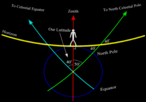
 I still use this minilesson in nearly every one of my presentations and for all ages. We have greatly improved the graphics used in this minilesson and I know you will like the results!
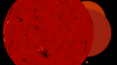 Like Solar System Scale, I use this minilesson frequently in most of my presentations, and we’ve revised it by adding a final graphic at the end which shows VY Canis Majoris in its entirety on the dome in one final scale shift.
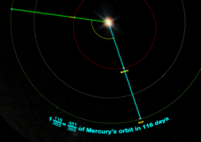 These are my favorite new additions in Volume 3! Each is a separate minilesson and carefully steps the audience through how Copernicus disentangled synodic periods of the planets into their sidereal periods around the Sun! Although very few people have ever been taught this concept, it’s very straightforward and illuminating when you see it on the dome. Test one out for yourself and you’ll be hooked!
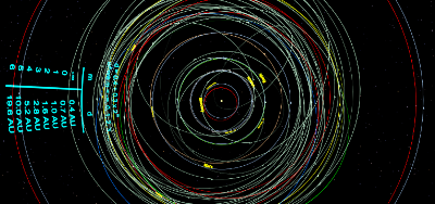 We often mention this infamous “Law” in our astronomy classes, so I wanted to present it in a historical fashion to demonstrate what effect it had on astronomer’s thinking when the Solar System was being explored and new planets being discovered. It’s the perfect example of a mathematical oddity that may or may not be scientifically meaningful. I think you will find it a fascinating subject as presented on the dome in this minilesson!