There is an upcoming event in the evening sky that is worth notifying your colleagues about on social media this week. Venus is going to pass in front of the Pleiades star cluster on Friday, April 3rd. The neat thing about it is that this happens every 8 years, to the day. You can simulate it on SciDome in Starry Night.
Venus is the brightest object in the evening sky other than the Moon this month, and it is provoking lots of UFO reports. Venus is also getting closer to Earth, so its apparent size is growing. Venus is also starting to turn into a crescent as it gets between the Earth and the Sun. It is a fascinating object to observe through small binoculars, especially when the Pleiades are also visible in the same binocular field of view.
Venus orbits the Sun every 225 days, but the Earth orbits the Sun as well, and it takes more than a year for Venus to catch up to the Earth and pass us. Venus returns to the same position with respect to the Earth every 8/5ths (or 1.6) of a year, or 584 days. Because it’s not equal to a year, when Venus returns after 584 days, it’s not in position against the same background stars. However, the lowest integer multiple of 1.6 is 8, so Venus does appear against the same background stars on the date when it passes the Earth every 8 years (although a backwards drift of 2 days per 8 years accumulates.)
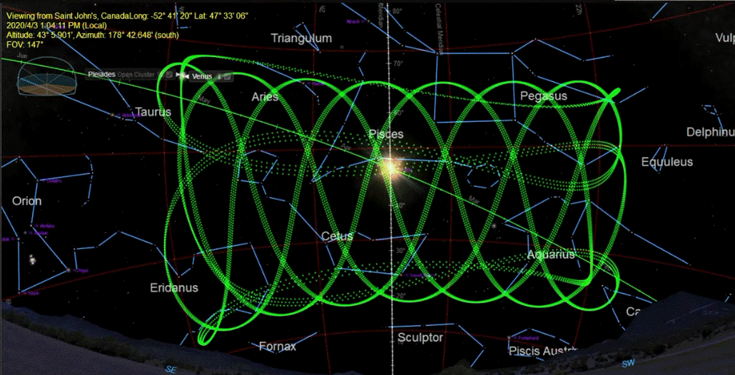
We’re familiar with the analemma, the figure-8 pattern the Sun draws on the sky if you animate Starry Night forward in steps of 1 day at noon. Venus also has an analemma, but it’s a spirograph pattern instead of a figure-8 because its Synodic period repeats five times over the course of those 8 years. This spirograph pattern of Venus’s Local Path at 1-day intervals in Starry Night is really cool.
The Synodic Period of Venus is covered in depth in David Bradstreet’s Fulldome Curriculum Vol. 3 minilesson “Synodic Period of Venus”.
The Pleiades is the brightest star cluster that happens to be on the Ecliptic plane, so it can periodically be occulted by the Moon, and the planets sometimes pass through it. Venus passes by the Pleiades every 8/5ths of a year too, although sometimes it passes by when the Pleiades is near the Sun in May, and sometimes when the Pleiades is in the predawn sky in late summer, and sometimes it passes by the Pleiades twice because it has a retrograde loop. The accumulating 2-day error also means that Venus’s path through the Pleiades is never quite the same with each 8-year interval, and the event is a coincidence that doesn’t look so perfect if you dial it back way into the past, or well into the future. But different dates become prominent for Venus meeting the Pleiades instead.
Venus’s greatest meeting in the sky is the Transit of Venus across the face of the Sun, which is very rare, and the Transit of Venus is also affected by that accumulating drift. Venus was in front of the Sun on June 8th, 2004 and again on June 6th, 2012, but another Transit will not happen again on June 4th, 2020 (but it will be close!) The next Transit of Venus will be on December 10th, 2117.
The first time I observed Venus in the Pleiades was on April 3rd, 1996, and I recommend you look up that date in Starry Night especially. Also on that date in the evening there was a total lunar eclipse in the eastern sky, and also the bright Comet Hyakutake was in the western sky just a few degrees away from the Pleiades.
So please make your community aware of the coincidence of Venus and the Pleiades this week, so they can look up again on April 3rd of 2028 and remember what they were doing 8 years earlier.
I hope you’ve heard about the Starlink constellation of satellites that is being put into orbit this year by SpaceX. Starlink is a global network that will provide satellite internet services with better speed and lower latency than current satellite internet. The difference is that instead of being located in the geosynchronous satellite belt 36,000 km above the Equator, the first wave of Starlink satellites orbit 550 km above Earth’s surface in a web of inclined planes.
362 Starlink satellites have been put into orbit so far, and SpaceX plans to continue to launch more, in batches of 60, until a complete “shell” of almost 1600 satellites is up there. Secondary constellations of thousands of Starlink satellites at different altitudes may follow. Starlink is not the only satellite internet provider that is planning a constellation like this: a company called Oneweb plans to launch a 650-unit constellation. SpaceX’s advantage over other providers is that they also own the rockets they are using to loft Starlink, and they can re-use those rockets several times.
In this case, the rocket scientists and the astronomers do not always get along. Thousands of extra satellites in low Earth orbit represent interference for optical astronomy, especially during local summer when satellites are in daylight for longer periods of night at Earth’s surface. These spacecraft could cause a wave of UFO reports. Some of us remember the beginning of the Iridium satellites and their bright “flares”, and comparable concerns we had for their effect on astronomy. Iridium has now gone away, but Starlink may produce more interference. SpaceX has demonstrated techniques to make the satellites dimmer and to minimize interference with astronomers in future.
Various K-band radio communications used by Starlink could also cause interference for radio astronomy. Also, the sheer number of new satellites poses a problem for orbital debris collisions, and SpaceX is implementing some new kind of collision avoidance scheme to avoid the possibility of a “Kessler Syndrome“, in which a chain reaction of collisions between satellites could make low Earth orbit unusable.
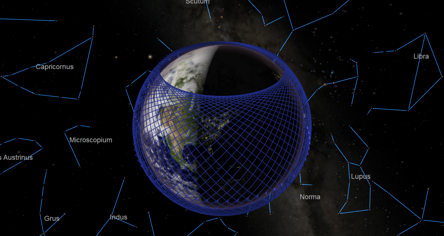
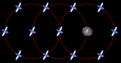
Although most of the Starlink constellation hasn’t been put into orbit yet, we know that the 1,584 satellites that are going up will be split into 72 different planes of 22 spacecraft each. I did a little extrapolation from the spacecraft already in orbit and generated a satellites file that Starry Night can use that simulates what these spacecraft will look like in the planetarium sky once they are all in orbit.
These Starlinks have imaginary names using a system “STARLINK AAAA, AAAB, AAAC…” This file doesn’t represent real satellites, and the method I used to make it requires replacing the satellites file already used by Starry Night. It is not hard to locate the files to be replaced and rename them for a while as we test out this file consisting of only Starlink satellites, so the generally useful data can be preserved. But if you are used to using views of the International Space Station or the Hubble Space Telescope in your Starry Night shows, that can’t be done at the same time as testing out this Starlink simulation.
The attached two files, Satellites.txt and SatelliteMagnitudes.txt, are text-parsable and represent the orbital elements of the satellites, and some data about how bright they are. The orbital elements are in the standard format used by NORAD, the US Air Force, etc., for this kind of data, known as Two Line Elements.
For the time being, let’s assume we are testing this on SciDome Preview Suite. Go to the following folder location on your Preview Suite computer:
C:\ProgramData\Simulation Curriculum\Starry Night Prefs\Sky Data
If you can’t see the ProgramData folder, the only problem is the ability to see hidden folders. Please contact me for advice. The Sky Data folder should already include, among other things, an original Satellites.txt and SatelliteMagnitudes.txt. Rename these files by adding a single character like a % or ^, and Starry Night won’t recognize them. Copy the two new files into this folder, and the next time Preview Suite boots up, it will load with the Starlink satellites instead of the usual ones. These satellites can be highlighted on the Preflight side and should become visible on the Renderbox side of Preview Suite at the same time.
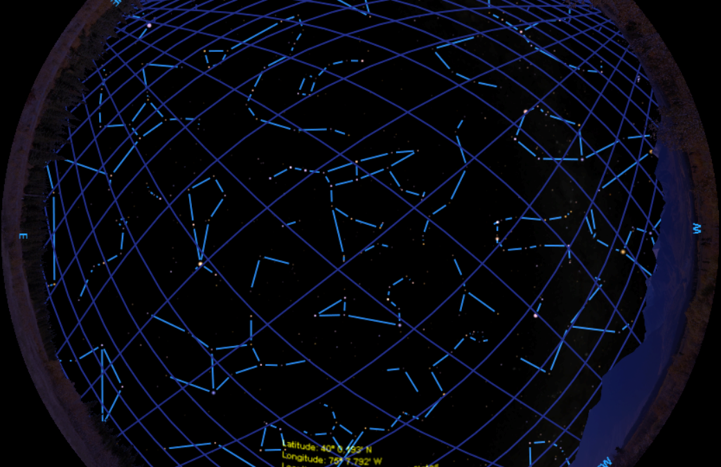
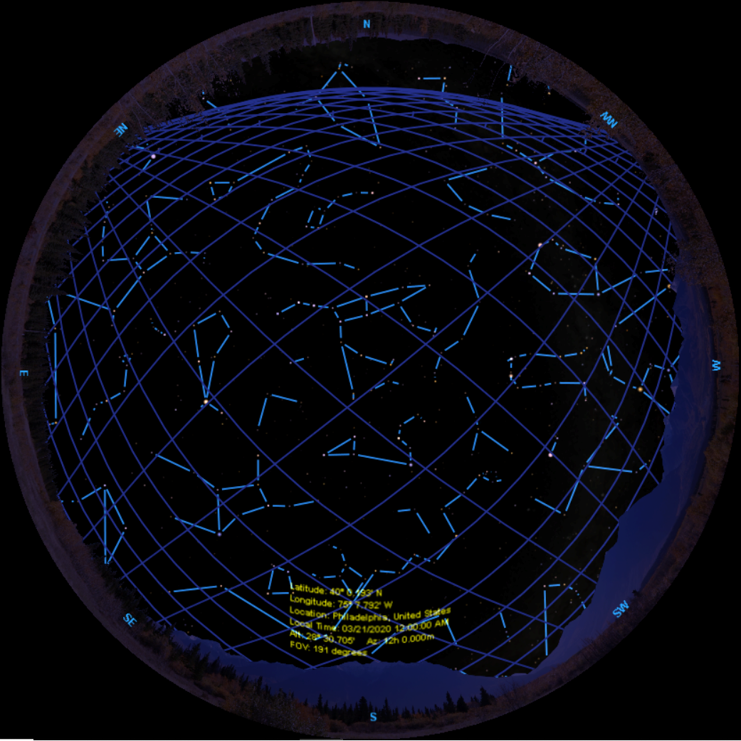
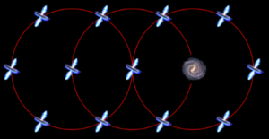
In these images, don’t think of the blue lines as real. They are just Starlinks with the orbit lines turned on. Think of each blue line segment as the path of each Starlink over the course of about 30 seconds, each blue diamond representing four of them.
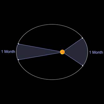
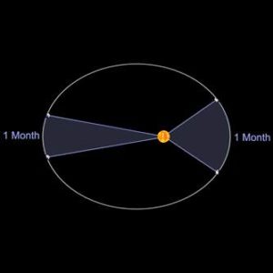
Recently Spitz (thanks to Software Architect, Clint Weisbrod) implemented new guide lines in Starry Night, graphically linking the Sun and planets (see the fall 2018 Spitz Newsletter and the Copernican Method). This inspired me to consider an animated, user-controllable version depicting Kepler’s Second Law. I have already implemented static images created by Steve Sanders (Eastern University’s Observatory Administrator) for teaching Kepler’s Second Law in Volume 2 of the Spitz Fulldome Curriculum, but static images pale in comparison to animations depicting the same concept.
Figure 1 – Kepler’s Second Law from FDC Volume 2
Kepler’s Second Law states that a radius vector connecting a planet to the Sun will sweep out equal areas in equal intervals of time. This paradigm-shattering result enabled the understanding of how planets change velocities in an orderly and systematic fashion (they are actually conserving angular momentum, but that realization would have to wait for Newton). Historic models mimicking the changing speeds of planets were complex and impressive but completely unwieldy when it came to calculations. They were also inaccurate.
What we devised (to be included in Fulldome Curriculum Volume 4) is a new Starry Night feature allowing Kepler’s Second Law to be illustrated for bodies in the solar system (planets, moons around planets, asteroids, comets, etc.), as well as exoplanets around their parent star. The feature allows operators to make a real-time graphical version of the sweeping sections of orbits.
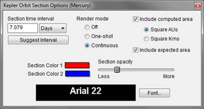
The controls for making Kepler Orbits are shown below:
The operator can enter time intervals for orbital segments (and we included a “Suggest Interval” function, which I almost always use, so beginning users have help in creating the segments). We can show individual orbital areas, and label the results.
Figure 2 – Kepler Orbit Section option dialog for Mercury
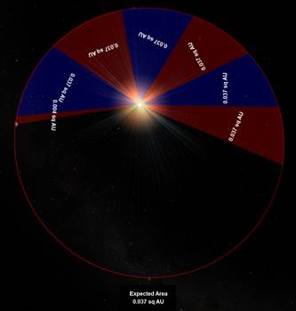
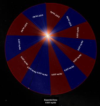
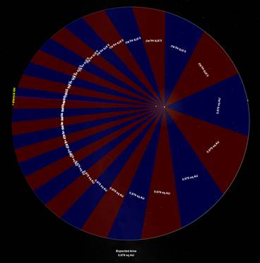
Figure 3a shows the result of running time for Mercury and Figure 3b displays the completed orbit. The numbers in each orbit segment are the numerically integrated areas of the segments, each of which is being calculated for the exact time interval set in the input box of Figure 2.
Figure 3a – Mercury beginning to draw Kepler Orbit sections in 7 day intervals
Figure 3b – Mercury completed Kepler Orbit sections in 7 day intervals
Note the Expected Area displayed at the bottom of the figures. This is the analytically calculated area for an orbital segment for Mercury given the time interval specified by the user. You may think, “Of course they are the same.” If you know anything about numerical analysis, it’s quite impressive that the numerical integration techniques implemented in this routine are accurate enough to reproduce the analytical prediction, i.e., validating Kepler’s Second Law.
We are so used to seeing equations predict outcomes that we’ve lost the astonishment of Kepler and Renaissance scientists for the precise nature of the universe, that it could be accurately modeled by mathematical equations!
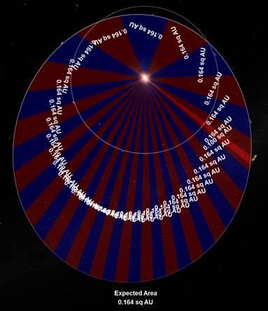
Let’s take a look at this feature for Halley’s Comet. Because of the extreme eccentricity typical of comets, we’ve only displayed the perihelion passage of this body, as illustrated in Figure 4.
Figure 4 – Perihelion passage of Halley’s Comet in 1986
Figure 5 displays the eccentric (0.56) Venus orbit-crossing asteroid 27 Apollo around the Sun. Venus’ orbit is shown to scale.
Figure 5 – The orbit of the Venus orbit-crossing asteroid 27 Apollo
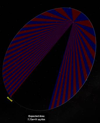
Figure 6 displays the very eccentric (0.75) orbit of Nereid, a moon of Neptune. I purposely didn’t display the numerically calculated areas to show what that looks like, i.e., to clean up the display.
Figure 6 Nereid’s orbit around Neptune, with an eccentricity of 0.75.
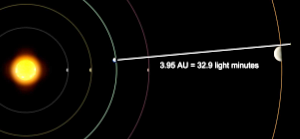
As a final example, Figure 7 displays the orbit of the exoplanet HD 87646b. It has an eccentricity of 0.500, an orbital period of 674 days and a semimajor axis of 1.580 AU.
Figure 7 – The orbit of exoplanet HD 87646b.
I sincerely hope that this upcoming new feature in SciDome excites audiences as much as it does all of us who have worked on implementing it! I also am extremely hopeful that when audiences see Kepler’s Second Law in action that they will finally be able to understand more fully what is meant by it.
Tomorrow, Friday, will be the 50th anniversary of the launch of Apollo 8, the first crewed space flight to orbit the Moon. You can simulate Apollo 8, and the other eight Apollo missions that went to the Moon, on your SciDome.
Apollo 8 mission patch, showing the “figure 8” path the spacecraft travelled from the Earth to the Moon
First, make sure that ‘Space Missions’ are checked to be visible in your View Options pane. If you type in ‘Apollo’ in the Starry Night search engine pane, each mission will come up, and you can break each one down by “Mission Path segments” that each describe a phase of flight, and look at the Command Module and Lunar Module separately at relevant points.
These missions can only be seen when Starry Night is displaying the right time between 1968 and 1972, which you can get by right-clicking on the mission you want and selecting “Set Time to Mission Event…” and picking “Launch”, for example. The best way to see the mission path of Apollo is to be looking at it from well above the Earth’s surface, with ‘Hover as Earth Rotates’ set so that the Earth’s surface can rotate underneath you and the fixed stars stay fixed on the dome.
Apollo 8 follows a curving path out from the Earth to the Moon, orbits around the Moon ten times, and then returns to the Earth. The different mission path segments are different colors.
You can see that the spacecraft orbits around the Moon from lunar west to lunar east. However, when we look up at Apollo’s path around the Moon it appears to be opposite the path that spacecraft orbit the Earth, even though everything launched from Cape Canaveral also goes towards the east. The Apollo spacecraft were launched into a figure-eight trajectory, so the “patching of conics” that reverses the frame of reference is like when two people shake hands on their right side. From one person’s point of view the other person is shaking their left hand, even though both participants are using their right.
The Apollo spacecraft and the Saturn V rocket are rendered in 3D in Starry Night if you go to them and look at them up close. The Apollo 8 spacecraft is pointed at the Earth by default.
The famous “Earthrise” photo was taken at the beginning of the fourth orbit, on December 24th, 1968, at about 16:25 Universal Time, as shown in SciDome. There is some question of which of the three astronauts – Commander Frank Borman, Command Module Pilot Jim Lovell, or “Lunar Module” Pilot Bill Anders – took the photo, and the question was resolved by Apollo historian Andrew Chaikin, who recounts his investigations in Smithsonian Magazine.
In Starry Night Preflight’s ‘SkyGuide’ pane there is a section on the Apollo missions, and Apollo 8 has 13 sub-headings that go into phases of flight like the Earthrise photo in some detail. Each subheading calls up a Starry Night application favourite scene that describes that phase of flight, with some text and images that appear in the SkyGuide pane.
Nicolaus Copernicus’ (1473 – 1543) paradigm-changing work de Revolutionibus Orbium Coelestium (On the Revolutions of the Celestial Spheres) famously laid the groundwork for the overthrow of the geocentric universe that had held sway for millennia. But what many people are not aware of is that Copernicus’ heliocentric system allowed for the first scale model of the entire known solar system in terms of the size of the Earth’s orbital radius.
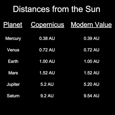
What I find most incredible is that the values he determined, despite assuming incorrectly that the planets’ orbits must be circular with the planets traveling at constant orbital speed, are very close to the modern-day measurements (shown in Table 1).
In my never-ending quest to create meaningful and engaging planetarium curriculum, Clint Weisbrod and I have developed the ability to reproduce Copernicus’ method using SciDome and new features in Starry Night which allow us to do solar system geometry.
Table 1 – Results of Copernicus’ model versus modern values.
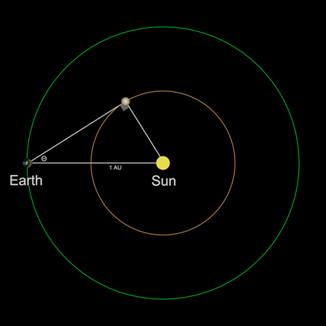
We begin by looking at the planets closer to the Sun than the Earth, the inferior planets Mercury and Venus (first denoted as such by Copernicus). Figure 1 shows the configuration for greatest elongation of Venus. By definition, this will occur when Venus appears to be the farthest away from the Sun as seen from Earth.
Via Euclid’s geometry we can prove that when Venus is at greatest elongation the angle at the position of Venus has to be exactly 90°. The line of sight from Earth to Venus must be tangent to Venus’ orbit, otherwise the line of sight would intersect the orbit in two places, both of which would display smaller angular separations from the Sun. The elongation angle θ is measured from the Earth as the angle between Venus and the Sun.
Knowing θ and that the angle at Venus is 90°, we can solve all sides of the triangle if we know one side of the triangle. Alas, we do not know any of the lengths, but if we define the distance from the Earth to the Sun (the hypotenuse) as 1 astronomical unit (1 AU), then we can immediately calculate the side of the triangle opposite the elongation angle θ as
Venus distance from Sun = (1 AU) sin θ
Figure 1 – The geometry (greatest elongation) of inferior planet distances from the Sun.
Figure 2 shows this configuration as seen from a top-down view of the Solar System in Starry Night using the new Copernican Method lines.
The value of the radius of the orbit of Venus (again assuming a circular orbit) is
Venus distance from Sun = (1 AU)sin(45.9°) = 0.72 AU
This is a remarkably accurate result, mostly due to Venus’ nearly circular orbit! The results for Mercury are not as accurate, but of course Mercury’s orbit is far from a circle. However, if enough measurements are made of multiple greatest elongations, the average will come out to be a fairly close estimate to the modern-day value.
Figure 2 – The Copernican Method lines for Venus in SciDome.
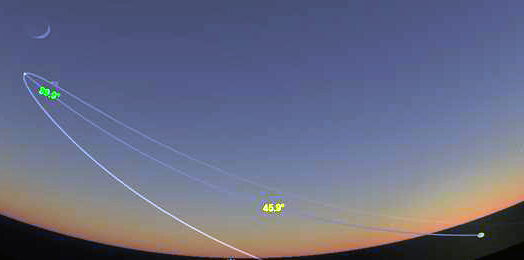
What’s awesome about the new feature in SciDome is that we can actually display the Copernican Method lines as seen from Earth as well as from space, as shown in Figure 3.
The line drawn between Venus and the Sun (just below the horizon) also displays the angular separation of the two bodies (45.9°) and the angle at Venus is the angle made between that line and the Earth’s line of sight (89.9° – close enough to 90° for government work).
The greatest elongation angle (45.9°) can be measured (in modern times) using a sextant (invented in 1715), so this new Copernican Method lines feature allows us to draw “sextant measurement lines” between the Sun and the planets.
Figure 3 – Venus’ greatest eastern elongation as seen from Philadelphia on August, 15, 2018.
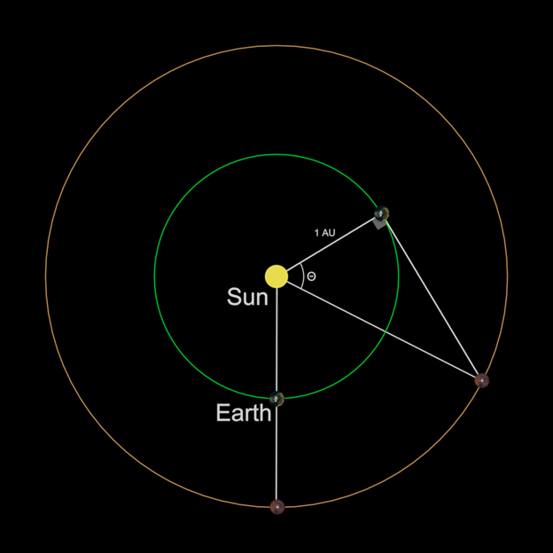
Determining the sizes of the orbits of the planets further from the Sun than the Earth—the superior planets—is not quite so straightforward. The method is explained below, remembering again that we’re assuming the orbits are all circular and the planets are moving at constant orbital speeds.
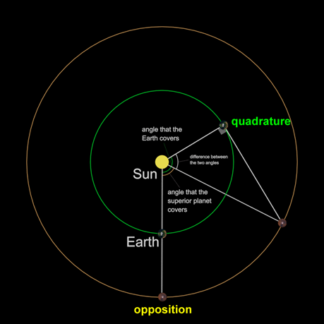
Figure 4 shows the geometry of the situation for superior planets. We begin by noting the date (Julian Date) of an opposition of the planet, when the planet and the Sun are on opposite sides of the Earth—the superior planet would rise when the Sun sets, and be highest in the sky (on your local meridian) at midnight. We then wait and observe the planet until it is 90° from the Sun, a position Copernicus defined as quadrature.
We calculate the number of days that have passed since opposition, and this will allow us to calculate how many degrees each planet has traversed in their respective orbits. For example, the Earth takes 365.2422 days to cover 360° (again, we’re assuming circular orbits and constant orbital velocity) so it will move
Figure 4 – The geometry of measuring the size of the orbits of the superior planets.
A similar calculation can be done for all the planets since Copernicus had calculated the sidereal periods of all the visible planets (see the Synodic Periods minilessons in Volume 3 of the Fulldome Curriculum). For example, Jupiter’s sidereal period is 4332.59 days yielding an angular rate of travel in its orbit of 0.0831 deg/day.
Since we know how many days it took for the planets to reach quadrature from opposition, we can immediately calculate how many degrees each planet traveled in their respective orbits. The Earth will travel a greater angle in its orbit in this time, and the difference between these two angles is the angle θ shown in Figure 5.
Assuming that the distance from Earth to the Sun is 1 AU, we can calculate the distance from the Sun to Jupiter (the hypotenuse of the triangle in Figure 5) as
So, what Earth observers would need to do is to measure the number of days from the opposition of a planet to the next quadrature, calculate the difference in degrees traveled between the two planets, and then take the reciprocal of the cosine of that angle to calculate the superior planet’s distance from the Sun.
Figure 5 – The quadrature triangle to solve for Jupiter’s distance from the Sun.
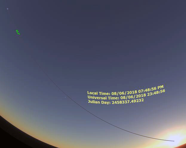
In the case of Jupiter, one set of measurements placed opposition on May 9, 2018 (JD 2458247.75) and the following quadrature on August 6, 2018 (JD 2458337.492), for a difference in days of 89.74. This value, multiplied by the difference in angular velocities between Earth and Jupiter, yielded a θ = 81.0°. This resulted in an orbital radius for Jupiter of 6.41 AU, whereas the modern value is 5.20 AU (a 23% difference). The view from Earth of this quadrature is shown in Figure 6.
At first glance, this value seems to be significantly off from the modern value…and it is! Have we made a mistake, or is this yet another opportunity to encourage our students to think? What assumptions have we made that are probably not accurate? We (as did Copernicus) assumed circular orbits and constant orbital velocities, and neither of these assumptions is correct for any of the planets!
So how can we use this method and the (wrong) assumption of circular orbits and constant orbital velocities to arrive at relatively accurate values for the sizes of the superior planets’ orbits?
The answer is to take multiple measurements over at least one orbital cycle of the planet in order for the answers to average out to some median value which indeed will approach the modern-day value. I did this for Jupiter taking 11 successive opposition-quadrature pairs over one 11-year cycle of its orbit from 2007 to 2018. When I averaged these 11 determinations I obtained a value of 5.46 AU, an error of only 5% from the modern value.
Don’t see this as a problem but rather as a very teachable moment for your students. You might challenge them as a class to take multiple measurements of successive opposition and quadrature pairs and they can watch for themselves how the values average out to close to the modern-day value. They can see for themselves how the errors introduced by our assumptions of circular orbit and constant orbital velocities can be minimized (but not eliminated) by multiple observations.
It’s appropriately mind-blowing to see the genius of Copernicus through these observations that your students can now undertake for themselves in the SciDome planetarium! They will gain a much greater understanding of how Copernicus created his solar system scale model, as well as see how these measurements could actually be made from the ground.
Figure 6 – The quadrature of Jupiter as seen from Philadelphia on August 6, 2018.
I’m excited to announce that Volume 3 of the Spitz Fulldome Curriculum is being released to all SciDome users, and will of course be automatically incorporated into all future SciDome installations. We thought that this would be an opportune time to give a very brief overview of what’s contained in this volume. There are several revisions to previous minilessons as well as several all new offerings:
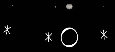
Galilean Moons
This minilesson gives 26 examples (in order of date) of Galileo’s first observations of the four major moons of Jupiter during the winter of 1610. The actual configuration of each night is beautifully displayed on the dome by Starry Night and then Galileo’s sketch is presented directly underneath it so that your audience can compare the sketch to reality. You will be astonished at Galileo’s accuracy, as well as the restrictions of his poor optics and resolution that confined his work. My students enjoy these comparisons even more than I do!
North Celestial Pole (NCP) Altitude
My students always scratch their heads when presented with the idea that the North Celestial Pole is always the same number of degrees above your horizon as your latitude. This series of overlaying diagrams attempts to clearly lay out exactly why this is the case.
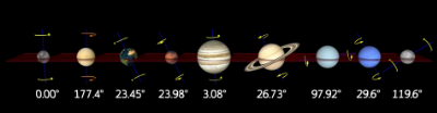
Planetary Tilts
Steve Sanders, Observatory Administrator at Eastern University and my right hand man, came up with this idea to beautifully illustrate the various planetary axis tilts side by side as well as their rotation periods. This animation is so impactful that the folks at ViewSpace used it in one of their presentations last year!
Quasars Fulldome
This is one of my all time favorite mind-blowing demonstrations! In a series of overlaying fulldome illustrations (again created by Steve Sanders), the second cosmological principle of the universe looking the same everywhere is demonstrated by using the appearance of quasars as seen from any galaxy, starting from the Milky Way. Your audience will be left awestruck when they discover that the Milky Way is a quasar as seen by a distant galaxy which to us looks like a quasar!
Roemer’s Method Revised
One of my favorite minilessons from Volume 1, we’ve revised this presentation with a new animation by Steve Sanders which very clearly shows the concept behind the light time effect and how Roemer was the first to demonstrate that the speed of light was finite and approximate its value. You can not only show this effect to your audience but make an incredibly precise and straightforward measurement from it of the speed of light!
Solar System Scale Revised
I still use this minilesson in nearly every one of my presentations and for all ages. We have greatly improved the graphics used in this minilesson and I know you will like the results!
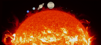
Stellar Sizes Revised
Like Solar System Scale, I use this minilesson frequently in most of my presentations, and we’ve revised it by adding a final graphic at the end which shows VY Canis Majoris in its entirety on the dome in one final scale shift.
Synodic Periods of Mercury, Venus, Mars and Jupiter
These are my favorite new additions in Volume 3! Each is a separate minilesson and carefully steps the audience through how Copernicus disentangled synodic periods of the planets into their sidereal periods around the Sun! Although very few people have ever been taught this concept, it’s very straightforward and illuminating when you see it on the dome. Test one out for yourself and you’ll be hooked!
Titius-Bode Rule
We often mention this infamous “Law” in our astronomy classes, so I wanted to present it in a historical fashion to demonstrate what effect it had on astronomer’s thinking when the Solar System was being explored and new planets being discovered. It’s the perfect example of a mathematical oddity that may or may not be scientifically meaningful. I think you will find it a fascinating subject as presented on the dome in this minilesson!
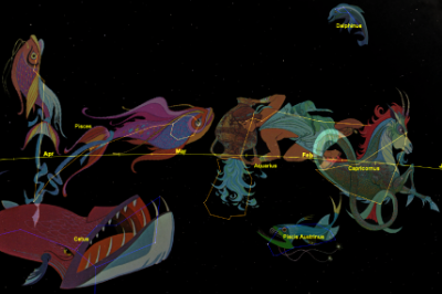
Watery Constellations
This little minilesson playfully depicts the fact that the region of the sky known as “The Sea” by the ancients has water-related constellations residing in it for a specific reason, namely that the Sun traversed this part of the sky during the rainy season in the Mediterranean. You will also be able to show your audience in a natural way that the position of the winter solstice used to be in Capricorn around 1000 BC, and hence that latitude parallel is called the Tropic of Capricorn.
Perhaps the greatest contribution to the official contents of Volume 3 is the availability of three unique fulldome interactive programs: Epicycles, Newton’s Mountain, and Tides. These three programs allow you to clearly demonstrate subjects which I have found extremely challenging for my students:
Epicycles shows many of the intricacies and systematics of the simplified Ptolemaic geocentric system and will alert your audiences to the vagaries of “saving the model at any cost.”
Newton’s Mountain is a 21st century interactive version of Newton’s attempt to explain exactly what an orbit is allowing you to show your audience in real time different orbits as a cannonball literally falls around the Earth.
Tides shows exactly why the Moon causes the water to bulge on either side of the Earth via differential gravitational forces as well as demonstrating that the bulge is not the same on both sides!
REQUIRES WINDOWS 7 ON THE RENDERBOX COMPUTER. Multi-projector systems must be based on Scaleable – not compatible with EasyBlend.
These three programs require purchase because of the many years of work which went into their development and implementation. They are now available for online purchase and immediate download:
I hope that you and your audiences thoroughly enjoy this latest addition to the Fulldome Curriculum, and that they will be helpful as you continue to strive to educate people in the subjects that we all love.


 This minilesson gives 26 examples (in order of date) of Galileo’s first observations of the four major moons of Jupiter during the winter of 1610. The actual configuration of each night is beautifully displayed on the dome by Starry Night and then Galileo’s sketch is presented directly underneath it so that your audience can compare the sketch to reality. You will be astonished at Galileo’s accuracy, as well as the restrictions of his poor optics and resolution that confined his work. My students enjoy these comparisons even more than I do!
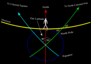
 I still use this minilesson in nearly every one of my presentations and for all ages. We have greatly improved the graphics used in this minilesson and I know you will like the results!
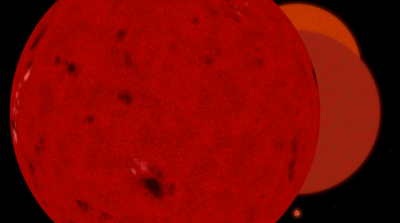 Like Solar System Scale, I use this minilesson frequently in most of my presentations, and we’ve revised it by adding a final graphic at the end which shows VY Canis Majoris in its entirety on the dome in one final scale shift.
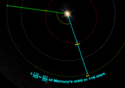 These are my favorite new additions in Volume 3! Each is a separate minilesson and carefully steps the audience through how Copernicus disentangled synodic periods of the planets into their sidereal periods around the Sun! Although very few people have ever been taught this concept, it’s very straightforward and illuminating when you see it on the dome. Test one out for yourself and you’ll be hooked!
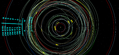 We often mention this infamous “Law” in our astronomy classes, so I wanted to present it in a historical fashion to demonstrate what effect it had on astronomer’s thinking when the Solar System was being explored and new planets being discovered. It’s the perfect example of a mathematical oddity that may or may not be scientifically meaningful. I think you will find it a fascinating subject as presented on the dome in this minilesson!