50 years ago this evening, the Apollo 13 spacecraft had its great “Houston, we’ve had a problem” moment. Apollo 13 is rendered in SciDome Preview Suite, with models representing the spacecraft both before and after panel #4 on the service module was blown off by the exploding oxygen tank.
Apollo 13 has been well-documented in several different media, and you may already have recommended your regular audience should check out the ‘Apollo 13’ movie, which we all love despite a few times it took dramatic license and presented a story that was a little more dramatic than the real thing. The most accurate representation of Apollo 13 now is the website www.apolloinrealtime.org, which is presenting a stereo mix of the astronauts’ and mission control’s audio loops, with scripts, images, movie clips and diagrams in real time.
The simplest way of looking at Apollo 13 in Preview Suite is to click on the hamburger icon on the leftmost pane and select ‘SkyGuide’. SkyGuide is a simple set of automations that presents an a la carte set of scenes, with descriptive text on the Preflight side. There is a ‘Space Missions’ button on the SkyGuide pane, with Apollo 13 as an option inside. The available Apollo 13 scenes are as follows:
Introduction
Launch into Earth Orbit
Trans-lunar injection – on the way to the Moon
View of the Earth
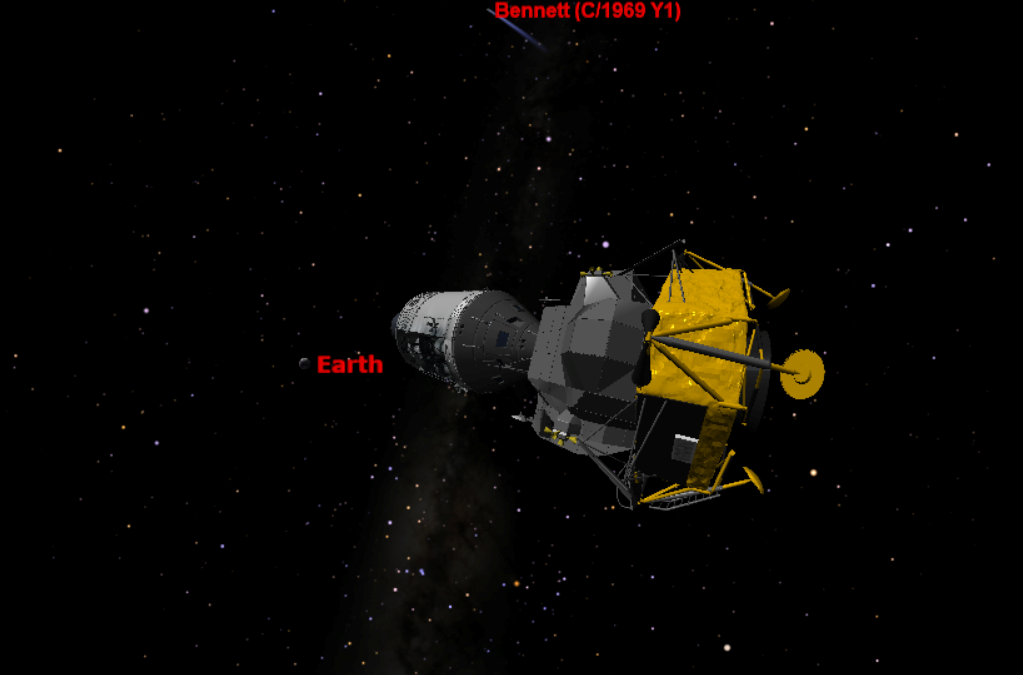
The accident
Around the Moon
Looking back at the Moon
The Service Module
The Lunar Module
Lessons learned
When you load one of these scenes, you may notice that they are zoomed in more than usual. This whole series was ported over from a different version of Starry Night, and may not be presented with the standard planetarium hemispherical view. At upper right are magnification controls, and you can use these to zoom out to the full field of view. You can also use “+” and “-” keystrokes to zoom in and out. The maximum field of view is the best dome view.
A few minutes before the oxygen tank explosion, which happened 50 years ago tonight at 10:07 PM EST (because they didn’t have daylight saving time until after the last Sunday in April at that time), just at the top of the hour, the astronauts were discussing orienting the spacecraft so that they could observe Comet Bennett, which was the 2nd-brightest comet visible in the 1970s, and just past its peak brightness at that time. Comet Bennett is not loaded in Preview Suite, but you can add it using the same guidelines I included in the most recent comet e-mail. Comet Bennett’s orbital elements can be entered into Starry Night as follows, with data from the JPL website:
Name: Bennett (C/1969 Y1)
e=0.996193
q=0.537606
i=90.0394
node=2246574
peri=354.1460
tp=2440665.5446
Epoch=2440680.5
The Odyssey command module which brought the three Apollo 13 astronauts back to Earth safely is on display at the Kansas Cosmosphere in Hutchinson, KS.
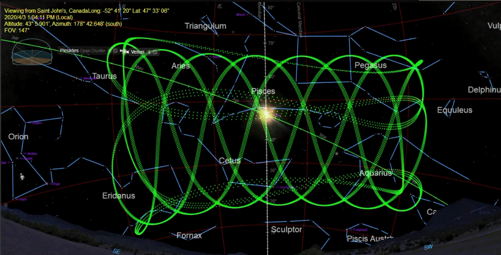
There is an upcoming event in the evening sky that is worth notifying your colleagues about on social media this week. Venus is going to pass in front of the Pleiades star cluster on Friday, April 3rd. The neat thing about it is that this happens every 8 years, to the day. You can simulate it on SciDome in Starry Night.
Venus is the brightest object in the evening sky other than the Moon this month, and it is provoking lots of UFO reports. Venus is also getting closer to Earth, so its apparent size is growing. Venus is also starting to turn into a crescent as it gets between the Earth and the Sun. It is a fascinating object to observe through small binoculars, especially when the Pleiades are also visible in the same binocular field of view.
Venus orbits the Sun every 225 days, but the Earth orbits the Sun as well, and it takes more than a year for Venus to catch up to the Earth and pass us. Venus returns to the same position with respect to the Earth every 8/5ths (or 1.6) of a year, or 584 days. Because it’s not equal to a year, when Venus returns after 584 days, it’s not in position against the same background stars. However, the lowest integer multiple of 1.6 is 8, so Venus does appear against the same background stars on the date when it passes the Earth every 8 years (although a backwards drift of 2 days per 8 years accumulates.)
We’re familiar with the analemma, the figure-8 pattern the Sun draws on the sky if you animate Starry Night forward in steps of 1 day at noon. Venus also has an analemma, but it’s a spirograph pattern instead of a figure-8 because its Synodic period repeats five times over the course of those 8 years. This spirograph pattern of Venus’s Local Path at 1-day intervals in Starry Night is really cool.
The Synodic Period of Venus is covered in depth in David Bradstreet’s Fulldome Curriculum Vol. 3 minilesson “Synodic Period of Venus”.
The Pleiades is the brightest star cluster that happens to be on the Ecliptic plane, so it can periodically be occulted by the Moon, and the planets sometimes pass through it. Venus passes by the Pleiades every 8/5ths of a year too, although sometimes it passes by when the Pleiades is near the Sun in May, and sometimes when the Pleiades is in the predawn sky in late summer, and sometimes it passes by the Pleiades twice because it has a retrograde loop. The accumulating 2-day error also means that Venus’s path through the Pleiades is never quite the same with each 8-year interval, and the event is a coincidence that doesn’t look so perfect if you dial it back way into the past, or well into the future. But different dates become prominent for Venus meeting the Pleiades instead.
Venus’s greatest meeting in the sky is the Transit of Venus across the face of the Sun, which is very rare, and the Transit of Venus is also affected by that accumulating drift. Venus was in front of the Sun on June 8th, 2004 and again on June 6th, 2012, but another Transit will not happen again on June 4th, 2020 (but it will be close!) The next Transit of Venus will be on December 10th, 2117.
The first time I observed Venus in the Pleiades was on April 3rd, 1996, and I recommend you look up that date in Starry Night especially. Also on that date in the evening there was a total lunar eclipse in the eastern sky, and also the bright Comet Hyakutake was in the western sky just a few degrees away from the Pleiades.
So please make your community aware of the coincidence of Venus and the Pleiades this week, so they can look up again on April 3rd of 2028 and remember what they were doing 8 years earlier.
I hope you’ve heard about the Starlink constellation of satellites that is being put into orbit this year by SpaceX. Starlink is a global network that will provide satellite internet services with better speed and lower latency than current satellite internet. The difference is that instead of being located in the geosynchronous satellite belt 36,000 km above the Equator, the first wave of Starlink satellites orbit 550 km above Earth’s surface in a web of inclined planes.
362 Starlink satellites have been put into orbit so far, and SpaceX plans to continue to launch more, in batches of 60, until a complete “shell” of almost 1600 satellites is up there. Secondary constellations of thousands of Starlink satellites at different altitudes may follow. Starlink is not the only satellite internet provider that is planning a constellation like this: a company called Oneweb plans to launch a 650-unit constellation. SpaceX’s advantage over other providers is that they also own the rockets they are using to loft Starlink, and they can re-use those rockets several times.
In this case, the rocket scientists and the astronomers do not always get along. Thousands of extra satellites in low Earth orbit represent interference for optical astronomy, especially during local summer when satellites are in daylight for longer periods of night at Earth’s surface. These spacecraft could cause a wave of UFO reports. Some of us remember the beginning of the Iridium satellites and their bright “flares”, and comparable concerns we had for their effect on astronomy. Iridium has now gone away, but Starlink may produce more interference. SpaceX has demonstrated techniques to make the satellites dimmer and to minimize interference with astronomers in future.
Various K-band radio communications used by Starlink could also cause interference for radio astronomy. Also, the sheer number of new satellites poses a problem for orbital debris collisions, and SpaceX is implementing some new kind of collision avoidance scheme to avoid the possibility of a “Kessler Syndrome“, in which a chain reaction of collisions between satellites could make low Earth orbit unusable.
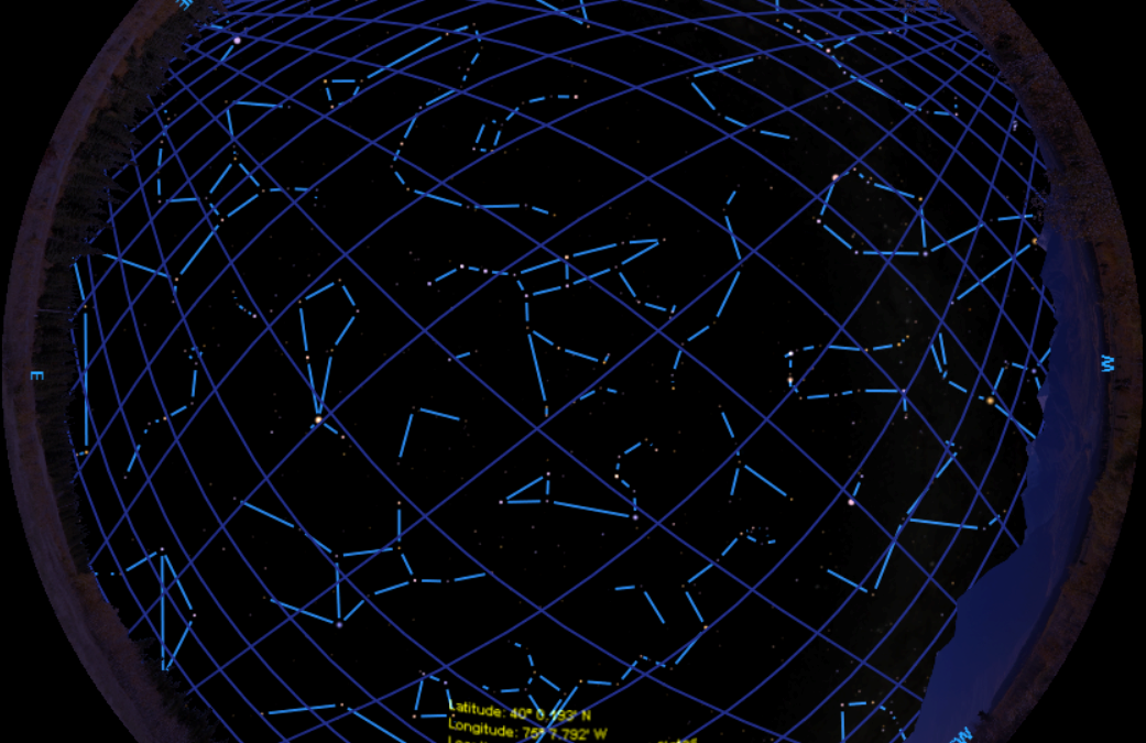
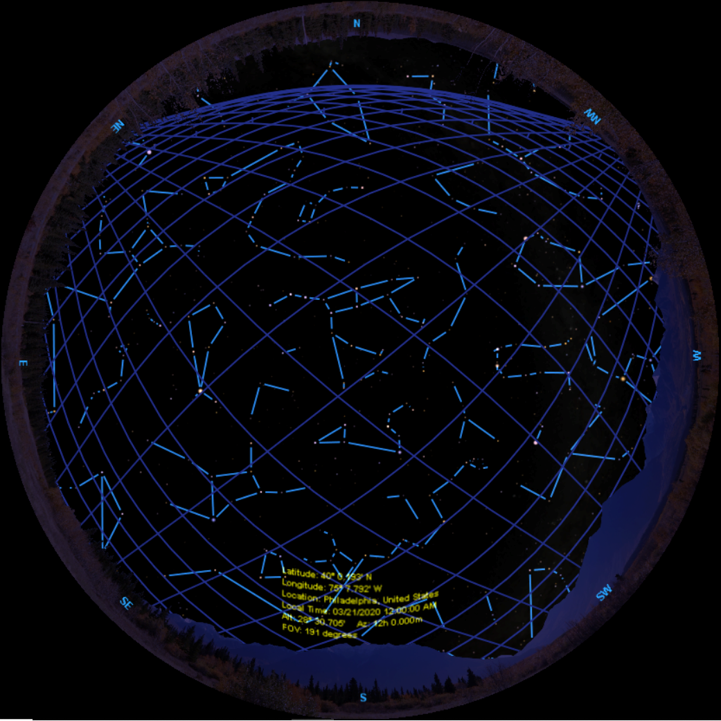
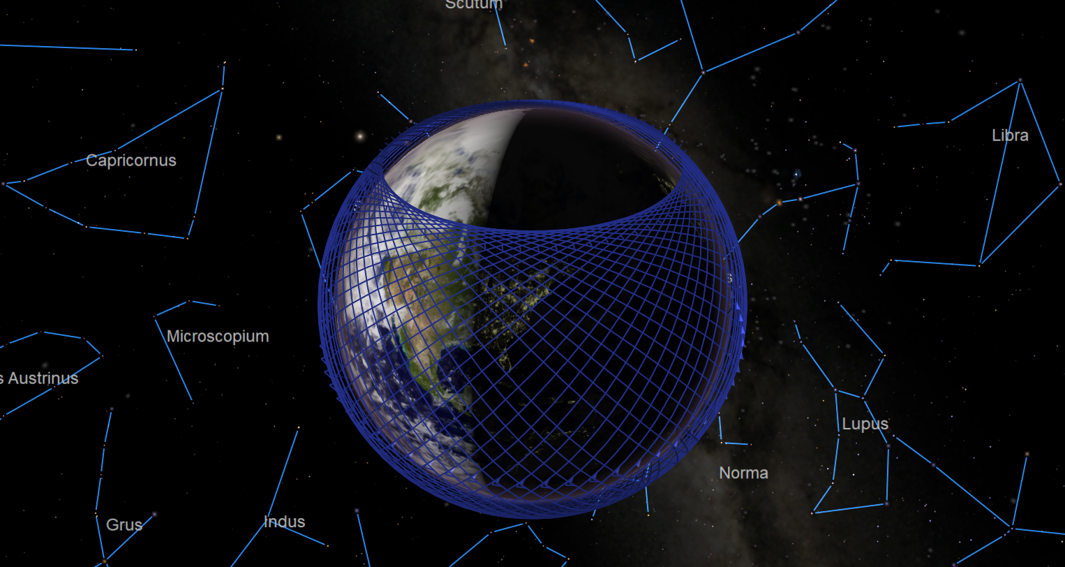
Although most of the Starlink constellation hasn’t been put into orbit yet, we know that the 1,584 satellites that are going up will be split into 72 different planes of 22 spacecraft each. I did a little extrapolation from the spacecraft already in orbit and generated a satellites file that Starry Night can use that simulates what these spacecraft will look like in the planetarium sky once they are all in orbit.
These Starlinks have imaginary names using a system “STARLINK AAAA, AAAB, AAAC…” This file doesn’t represent real satellites, and the method I used to make it requires replacing the satellites file already used by Starry Night. It is not hard to locate the files to be replaced and rename them for a while as we test out this file consisting of only Starlink satellites, so the generally useful data can be preserved. But if you are used to using views of the International Space Station or the Hubble Space Telescope in your Starry Night shows, that can’t be done at the same time as testing out this Starlink simulation.
The attached two files, Satellites.txt and SatelliteMagnitudes.txt, are text-parsable and represent the orbital elements of the satellites, and some data about how bright they are. The orbital elements are in the standard format used by NORAD, the US Air Force, etc., for this kind of data, known as Two Line Elements.
For the time being, let’s assume we are testing this on SciDome Preview Suite. Go to the following folder location on your Preview Suite computer:
C:\ProgramData\Simulation Curriculum\Starry Night Prefs\Sky Data
If you can’t see the ProgramData folder, the only problem is the ability to see hidden folders. Please contact me for advice. The Sky Data folder should already include, among other things, an original Satellites.txt and SatelliteMagnitudes.txt. Rename these files by adding a single character like a % or ^, and Starry Night won’t recognize them. Copy the two new files into this folder, and the next time Preview Suite boots up, it will load with the Starlink satellites instead of the usual ones. These satellites can be highlighted on the Preflight side and should become visible on the Renderbox side of Preview Suite at the same time.
In these images, don’t think of the blue lines as real. They are just Starlinks with the orbit lines turned on. Think of each blue line segment as the path of each Starlink over the course of about 30 seconds, each blue diamond representing four of them.
Just after midnight on January 1st, the New Horizons spacecraft will have its close encounter with the Kuiper Belt object Ultima Thule, also known as (486958) 2014 MU69. Since New Horizons flew by Pluto in July 2015 it has been preparing for this moment. Ultima Thule wasn’t even targeted until after the Pluto encounter was over, and it was only discovered in 2014.
Of course, the next thing is simulating the encounter in Starry Night. The first problem here is that the mission path provided for New Horizons in Starry Night doesn’t extend to the present day. However, the JPL HORIZONS service can provide updated state vectors, which I have put into the attached file New Horizons.xyz.
To get the updated mission path of New Horizons into your SciDome, download this zip, open it, and copy “New Horizons.xyz” into this folder on your Preflight computer running SciDome Version 7:
C:\ProgramData\Simulation Curriculum\Starry Night Prefs\Sky Data\Space Missions
This is a networked folder that exists on both Preflight and Renderbox computers, so the file only needs to be in one place in order to be accessible in both computers. If there is no “Space Missions” subfolder of this SkyData folder, you may have to create it. Although there will then be more than one version of the New Horizons file on your system, this one will take precedence.
Ultima Thule imagery captured by New Horizons
Next, we have to add Ultima Thule to Starry Night. I find the best way to do this is to right-click on the Sun and in the details window that pops up, select ‘New Asteroid…’ In the ‘Asteroid: Untitled’ window that pops up, enter the following data, which comes from the Minor Planet Center at Harvard:
Name: Ultima Thule
Mean Distance: 44.581400
Eccentricity: 0.041725
Inclination: 2.4512
Ascending Node: 158.9977
Arg of Pericentre: 174.4177
Mean Anomaly: 316.5508
Epoch: 2458600.5
Exit this window and answer the prompt, ‘Do you want to save changes…?’ with yes. The next time you quit Starry Night, this new object will be saved into a file called “User Planets.ssd” that lives on your Preflight computer, but is not automatically networked to the Renderbox. In order to get it to live on the Renderbox, you have to find “User Planets.ssd” and copy it into part of the Sky Data folder we looked at above.
Locate ‘User Planets.ssd’ in the following folder:
C:\Users\SPITZ\AppData\Local\Simulation Curriculum\Starry Night Prefs\Preflight\
Verify that this file was last modified on the date you are doing this work.
The destination the file should be copied to is:
C:\ProgramData\Simulation Curriculum\Starry Night Prefs\Sky Data\
If there is an older version of ‘User Planets.ssd’ in the destination, better save it to a safe location, just in case.
The Ultima Thule encounter could be a strange one. Pluto is about as big as the United States, from the 49th parallel to the Rio Grande, but Ultima Thule is only about as big as Nantucket Sound. Its shape has been worked out from occultations, and it looks elongated, not round. You can get more data about the mission to share from this blog entry from Emily Lakdawalla at the Planetary Society.
Tomorrow, Friday, will be the 50th anniversary of the launch of Apollo 8, the first crewed space flight to orbit the Moon. You can simulate Apollo 8, and the other eight Apollo missions that went to the Moon, on your SciDome.
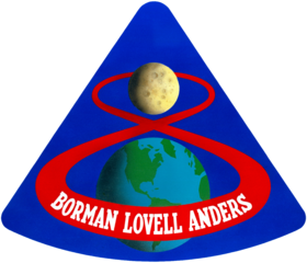
Apollo 8 mission patch, showing the “figure 8” path the spacecraft travelled from the Earth to the Moon
First, make sure that ‘Space Missions’ are checked to be visible in your View Options pane. If you type in ‘Apollo’ in the Starry Night search engine pane, each mission will come up, and you can break each one down by “Mission Path segments” that each describe a phase of flight, and look at the Command Module and Lunar Module separately at relevant points.
These missions can only be seen when Starry Night is displaying the right time between 1968 and 1972, which you can get by right-clicking on the mission you want and selecting “Set Time to Mission Event…” and picking “Launch”, for example. The best way to see the mission path of Apollo is to be looking at it from well above the Earth’s surface, with ‘Hover as Earth Rotates’ set so that the Earth’s surface can rotate underneath you and the fixed stars stay fixed on the dome.
Apollo 8 follows a curving path out from the Earth to the Moon, orbits around the Moon ten times, and then returns to the Earth. The different mission path segments are different colors.
You can see that the spacecraft orbits around the Moon from lunar west to lunar east. However, when we look up at Apollo’s path around the Moon it appears to be opposite the path that spacecraft orbit the Earth, even though everything launched from Cape Canaveral also goes towards the east. The Apollo spacecraft were launched into a figure-eight trajectory, so the “patching of conics” that reverses the frame of reference is like when two people shake hands on their right side. From one person’s point of view the other person is shaking their left hand, even though both participants are using their right.
The Apollo spacecraft and the Saturn V rocket are rendered in 3D in Starry Night if you go to them and look at them up close. The Apollo 8 spacecraft is pointed at the Earth by default.
The famous “Earthrise” photo was taken at the beginning of the fourth orbit, on December 24th, 1968, at about 16:25 Universal Time, as shown in SciDome. There is some question of which of the three astronauts – Commander Frank Borman, Command Module Pilot Jim Lovell, or “Lunar Module” Pilot Bill Anders – took the photo, and the question was resolved by Apollo historian Andrew Chaikin, who recounts his investigations in Smithsonian Magazine.
In Starry Night Preflight’s ‘SkyGuide’ pane there is a section on the Apollo missions, and Apollo 8 has 13 sub-headings that go into phases of flight like the Earthrise photo in some detail. Each subheading calls up a Starry Night application favourite scene that describes that phase of flight, with some text and images that appear in the SkyGuide pane.
Nicolaus Copernicus’ (1473 – 1543) paradigm-changing work de Revolutionibus Orbium Coelestium (On the Revolutions of the Celestial Spheres) famously laid the groundwork for the overthrow of the geocentric universe that had held sway for millennia. But what many people are not aware of is that Copernicus’ heliocentric system allowed for the first scale model of the entire known solar system in terms of the size of the Earth’s orbital radius.
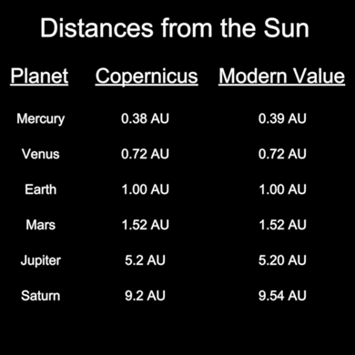
What I find most incredible is that the values he determined, despite assuming incorrectly that the planets’ orbits must be circular with the planets traveling at constant orbital speed, are very close to the modern-day measurements (shown in Table 1).
In my never-ending quest to create meaningful and engaging planetarium curriculum, Clint Weisbrod and I have developed the ability to reproduce Copernicus’ method using SciDome and new features in Starry Night which allow us to do solar system geometry.
Table 1 – Results of Copernicus’ model versus modern values.
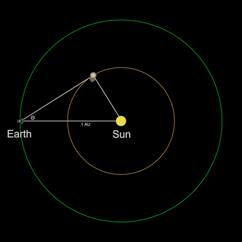
We begin by looking at the planets closer to the Sun than the Earth, the inferior planets Mercury and Venus (first denoted as such by Copernicus). Figure 1 shows the configuration for greatest elongation of Venus. By definition, this will occur when Venus appears to be the farthest away from the Sun as seen from Earth.
Via Euclid’s geometry we can prove that when Venus is at greatest elongation the angle at the position of Venus has to be exactly 90°. The line of sight from Earth to Venus must be tangent to Venus’ orbit, otherwise the line of sight would intersect the orbit in two places, both of which would display smaller angular separations from the Sun. The elongation angle θ is measured from the Earth as the angle between Venus and the Sun.
Knowing θ and that the angle at Venus is 90°, we can solve all sides of the triangle if we know one side of the triangle. Alas, we do not know any of the lengths, but if we define the distance from the Earth to the Sun (the hypotenuse) as 1 astronomical unit (1 AU), then we can immediately calculate the side of the triangle opposite the elongation angle θ as
Venus distance from Sun = (1 AU) sin θ
Figure 1 – The geometry (greatest elongation) of inferior planet distances from the Sun.
Figure 2 shows this configuration as seen from a top-down view of the Solar System in Starry Night using the new Copernican Method lines.
The value of the radius of the orbit of Venus (again assuming a circular orbit) is
Venus distance from Sun = (1 AU)sin(45.9°) = 0.72 AU
This is a remarkably accurate result, mostly due to Venus’ nearly circular orbit! The results for Mercury are not as accurate, but of course Mercury’s orbit is far from a circle. However, if enough measurements are made of multiple greatest elongations, the average will come out to be a fairly close estimate to the modern-day value.
Figure 2 – The Copernican Method lines for Venus in SciDome.
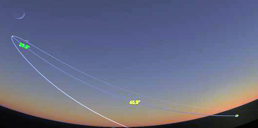
What’s awesome about the new feature in SciDome is that we can actually display the Copernican Method lines as seen from Earth as well as from space, as shown in Figure 3.
The line drawn between Venus and the Sun (just below the horizon) also displays the angular separation of the two bodies (45.9°) and the angle at Venus is the angle made between that line and the Earth’s line of sight (89.9° – close enough to 90° for government work).
The greatest elongation angle (45.9°) can be measured (in modern times) using a sextant (invented in 1715), so this new Copernican Method lines feature allows us to draw “sextant measurement lines” between the Sun and the planets.
Figure 3 – Venus’ greatest eastern elongation as seen from Philadelphia on August, 15, 2018.
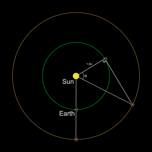
Determining the sizes of the orbits of the planets further from the Sun than the Earth—the superior planets—is not quite so straightforward. The method is explained below, remembering again that we’re assuming the orbits are all circular and the planets are moving at constant orbital speeds.
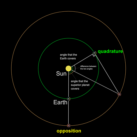
Figure 4 shows the geometry of the situation for superior planets. We begin by noting the date (Julian Date) of an opposition of the planet, when the planet and the Sun are on opposite sides of the Earth—the superior planet would rise when the Sun sets, and be highest in the sky (on your local meridian) at midnight. We then wait and observe the planet until it is 90° from the Sun, a position Copernicus defined as quadrature.
We calculate the number of days that have passed since opposition, and this will allow us to calculate how many degrees each planet has traversed in their respective orbits. For example, the Earth takes 365.2422 days to cover 360° (again, we’re assuming circular orbits and constant orbital velocity) so it will move
Figure 4 – The geometry of measuring the size of the orbits of the superior planets.
A similar calculation can be done for all the planets since Copernicus had calculated the sidereal periods of all the visible planets (see the Synodic Periods minilessons in Volume 3 of the Fulldome Curriculum). For example, Jupiter’s sidereal period is 4332.59 days yielding an angular rate of travel in its orbit of 0.0831 deg/day.
Since we know how many days it took for the planets to reach quadrature from opposition, we can immediately calculate how many degrees each planet traveled in their respective orbits. The Earth will travel a greater angle in its orbit in this time, and the difference between these two angles is the angle θ shown in Figure 5.
Assuming that the distance from Earth to the Sun is 1 AU, we can calculate the distance from the Sun to Jupiter (the hypotenuse of the triangle in Figure 5) as
So, what Earth observers would need to do is to measure the number of days from the opposition of a planet to the next quadrature, calculate the difference in degrees traveled between the two planets, and then take the reciprocal of the cosine of that angle to calculate the superior planet’s distance from the Sun.
Figure 5 – The quadrature triangle to solve for Jupiter’s distance from the Sun.
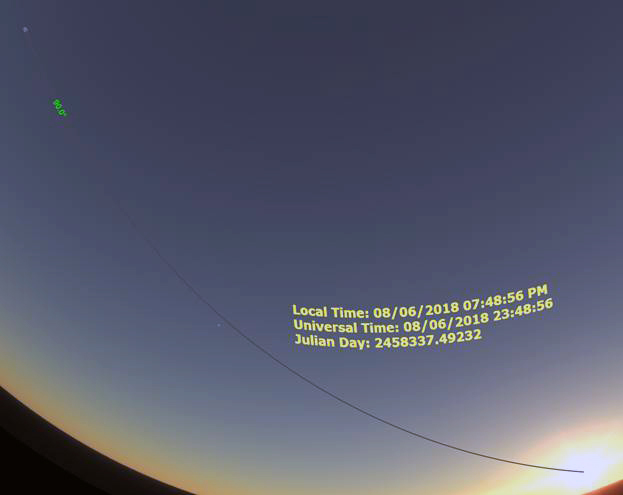
In the case of Jupiter, one set of measurements placed opposition on May 9, 2018 (JD 2458247.75) and the following quadrature on August 6, 2018 (JD 2458337.492), for a difference in days of 89.74. This value, multiplied by the difference in angular velocities between Earth and Jupiter, yielded a θ = 81.0°. This resulted in an orbital radius for Jupiter of 6.41 AU, whereas the modern value is 5.20 AU (a 23% difference). The view from Earth of this quadrature is shown in Figure 6.
At first glance, this value seems to be significantly off from the modern value…and it is! Have we made a mistake, or is this yet another opportunity to encourage our students to think? What assumptions have we made that are probably not accurate? We (as did Copernicus) assumed circular orbits and constant orbital velocities, and neither of these assumptions is correct for any of the planets!
So how can we use this method and the (wrong) assumption of circular orbits and constant orbital velocities to arrive at relatively accurate values for the sizes of the superior planets’ orbits?
The answer is to take multiple measurements over at least one orbital cycle of the planet in order for the answers to average out to some median value which indeed will approach the modern-day value. I did this for Jupiter taking 11 successive opposition-quadrature pairs over one 11-year cycle of its orbit from 2007 to 2018. When I averaged these 11 determinations I obtained a value of 5.46 AU, an error of only 5% from the modern value.
Don’t see this as a problem but rather as a very teachable moment for your students. You might challenge them as a class to take multiple measurements of successive opposition and quadrature pairs and they can watch for themselves how the values average out to close to the modern-day value. They can see for themselves how the errors introduced by our assumptions of circular orbit and constant orbital velocities can be minimized (but not eliminated) by multiple observations.
It’s appropriately mind-blowing to see the genius of Copernicus through these observations that your students can now undertake for themselves in the SciDome planetarium! They will gain a much greater understanding of how Copernicus created his solar system scale model, as well as see how these measurements could actually be made from the ground.
Figure 6 – The quadrature of Jupiter as seen from Philadelphia on August 6, 2018.
 50 years ago this evening, the Apollo 13 spacecraft had its great “Houston, we’ve had a problem” moment. Apollo 13 is rendered in SciDome Preview Suite, with models representing the spacecraft both before and after panel #4 on the service module was blown off by the exploding oxygen tank.
Apollo 13 has been well-documented in several different media, and you may already have recommended your regular audience should check out the ‘Apollo 13’ movie, which we all love despite a few times it took dramatic license and presented a story that was a little more dramatic than the real thing. The most accurate representation of Apollo 13 now is the website www.apolloinrealtime.org, which is presenting a stereo mix of the astronauts’ and mission control’s audio loops, with scripts, images, movie clips and diagrams in real time.
The simplest way of looking at Apollo 13 in Preview Suite is to click on the hamburger icon on the leftmost pane and select ‘SkyGuide’. SkyGuide is a simple set of automations that presents an a la carte set of scenes, with descriptive text on the Preflight side. There is a ‘Space Missions’ button on the SkyGuide pane, with Apollo 13 as an option inside. The available Apollo 13 scenes are as follows:
50 years ago this evening, the Apollo 13 spacecraft had its great “Houston, we’ve had a problem” moment. Apollo 13 is rendered in SciDome Preview Suite, with models representing the spacecraft both before and after panel #4 on the service module was blown off by the exploding oxygen tank.
Apollo 13 has been well-documented in several different media, and you may already have recommended your regular audience should check out the ‘Apollo 13’ movie, which we all love despite a few times it took dramatic license and presented a story that was a little more dramatic than the real thing. The most accurate representation of Apollo 13 now is the website www.apolloinrealtime.org, which is presenting a stereo mix of the astronauts’ and mission control’s audio loops, with scripts, images, movie clips and diagrams in real time.
The simplest way of looking at Apollo 13 in Preview Suite is to click on the hamburger icon on the leftmost pane and select ‘SkyGuide’. SkyGuide is a simple set of automations that presents an a la carte set of scenes, with descriptive text on the Preflight side. There is a ‘Space Missions’ button on the SkyGuide pane, with Apollo 13 as an option inside. The available Apollo 13 scenes are as follows: